American Scientist

Mathematical models and computer simulations usually begin as aids to understanding, introduced when some aspect of natural science proves too knotty for direct analysis. Facing an intractable problem, we strip away all the messy details of the real world and build a toy universe, one simple enough that we can hope to master it. Often, though, even the dumbed-down model defies exact solution or accurate computation. Then the model itself becomes an object of scientific inquiry—a puzzle to be solved.

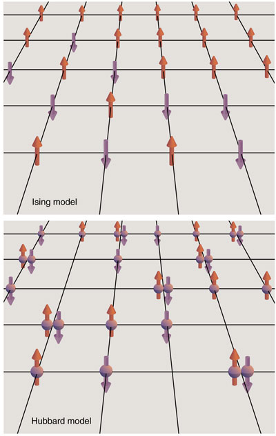
A good example is the Ising model in solid-state physics, which attempts to explain the nature of magnetism in materials such as iron. (I wrote about the Ising model in an earlier Computing Science column; see “The World in a Spin,” September–October 2000.) The Ising model glosses over all the intricacies of atomic structure, representing a magnet as a simple array of electron “spins” on a plain, gridlike lattice. Even in this abstract form, however, the model presents serious challenges. Only a two-dimensional version has been solved exactly; for the three- dimensional model, getting accurate results requires both algorithmic sophistication and major computer power.

One step up from the Ising model—in terms of realism and complexity—is something called the Hubbard model. Again the aim is to describe aspects of solid-state physics, including various kinds of magnetism as well as certain conductive and insulating materials, and maybe even the high-temperature superconductors that have stumped theorists since the 1980s. As in the Ising model, the Hubbard model puts electrons on a simple lattice, but in this case the electrons are allowed to hop from site to site. The model also insists on a quantum-mechanical treatment of the interactions between electrons. These two features make the Hubbard model a much harder nut to crack.

Except in the special case of a one-dimensional lattice, the Hubbard model has defied exact mathematical analysis. And computer simulations of Hubbard systems become painfully slow with any more than a few dozen electrons. Calculations are so difficult that no one knows for sure whether various Hubbard systems are conductive or insulating, or what their magnetic properties might be. This situation has led to an extraordinary new strategy for solving the model: putting it to the test of experiment. Several groups of physicists have built macroscopic replicas of the Hubbard lattice out of light waves and trapped atoms. Thus we come full circle, creating a physical analog of an abstract model that in turn represents another physical system.

Magnetic Attractions

At the most superficial level, the antics of electrons in solids seem easy enough to comprehend. A substance is conductive if at least some of its electrons are free to wander about; when every electron is tightly bound to an atom, the material is an insulator. Magnetic effects derive from the spin of the electron, which gives rise to a tiny magnetic dipole moment, like that of a bar magnet. The strongest form of magnetism (ferromagnetism) appears when nearly all the spins line up in the same direction.

Going beyond this level of understanding is not so easy. What property of a solid determines whether electrons are nomadic or frozen in place? Why do electron spins in iron and nickel adopt a parallel alignment whereas those of zinc and copper remain randomly oriented? A useful theory should also make quantitative predictions. For example, how does conductivity or magnetization vary as a function of temperature?

This last question brings us back to the Ising model, which was devised to explore the thermal properties of ferromagnets. If you heat a magnet to high temperature, the magnetization fades away. Then, when you allow the material to cool again, it regains its magnetic properties at a specific temperature called the Curie point (1,040 kelvins for iron). The transition is abrupt: A graph of magnetization as a function of temperature shows a discontinuity—a sharp kink—at the Curie point. Evidently there is a sudden transition from thermal chaos to magnetic order.

The Ising model was designed to capture the essential features of this behavior. The model was invented by the German physicist Wilhelm Lenz and investigated by his student Ernst Ising in the 1920s, at a time when the quantum theory of solids was still in its infancy. They represented the spin of an electron by a simple arrow constrained to point either up or down. Interactions of the spins were codified in two rules. First, pairs of adjacent spins prefer to point the same way, either both up or both down; there is an energy penalty whenever nearest-neighbor spins are antiparallel. Second, thermal fluctuations tend to mix up the spins, flipping them at random; thus orderly alignments are disrupted when the temperature rises.

Ising hoped to observe a sudden onset of magnetization, as in real ferromagnets. He analyzed a one-dimensional version of the model, in which the lattice is merely a line or a ring. Disappointingly, he found no discontinuous transition to a magnetized state at any temperature above absolute zero.

Ising believed that this negative result would carry over to higher dimensions as well, but a decade later other physicists found hints of magnetization in two dimensions. Then in 1944 Lars Onsager confirmed these results with an exact mathematical solution of the two-dimensional Ising model; his equation showed that magnetization in the planar spin system does indeed jump discontinuously at a nonzero critical temperature. For three dimensions no exact solution has ever been found, but computer simulations give unmistakable evidence of an abrupt phase transition.

The Ising model has gone on to become a kind of model for models. The same abstract structure—a lattice of sites, nearest-neighbor interactions, a variable at each site that takes on two discrete values—has served to describe not only magnets but also dozens of other physical systems, such as alloys (where the up and down spins represent atoms of two different elements) and gases (where the two states indicate the presence or absence of an atom). Ising-like models have even made their way into the social sciences, where they describe phenomena such as the emergence of racial segregation in housing patterns.

Meanwhile, despite all these diverse successes, the Ising model has not proved entirely satisfactory for its original purpose—as a tool for understanding ferromagnetism. In this application the model has two major weaknesses. First, spins in the Ising model are rigidly pinned to the lattice sites, but it turns out that some degree of electron mobility is crucial to many magnetic phenomena. Second, although the Ising model was inspired by quantum-mechanical ideas, it incorporates none of the peculiar rules and regulations that the quantum theory imposes on electrons. The Hubbard model addresses both of these issues.

The Crowded Dance Floor

The stage setting for the Hubbard model is the same as that of the Ising model: a simple lattice with cubic symmetry—a cartoon of a crystalline solid. But the Hubbard dancers are more acrobatic. As noted above, Hubbard electrons can jump from one lattice site to another. (The range of motion is usually limited to nearest-neighbor sites.) The electrons also interact with one another, experiencing mutual repulsion whenever two electrons land on the same site. Finally, the choreography of Hubbard electrons is subject to a special rule, the Pauli exclusion principle, a definitive element of quantum mechanics.

Think of the Pauli principle (named for the Austrian physicist Wolfgang Pauli) as a generalization of the commonsense notion that two objects cannot be in the same place at the same time. The quantum version says that no two particles can occupy exactly the same quantum state. If two electrons have the same energy, for example, they must differ in angular momentum or some other property. On the Hubbard lattice, the exclusion principle implies that if two electrons occupy the same site, they must have opposite spins. An obvious corollary is that no site can ever accommodate more than two electrons, since at least two of them would have the same spin.

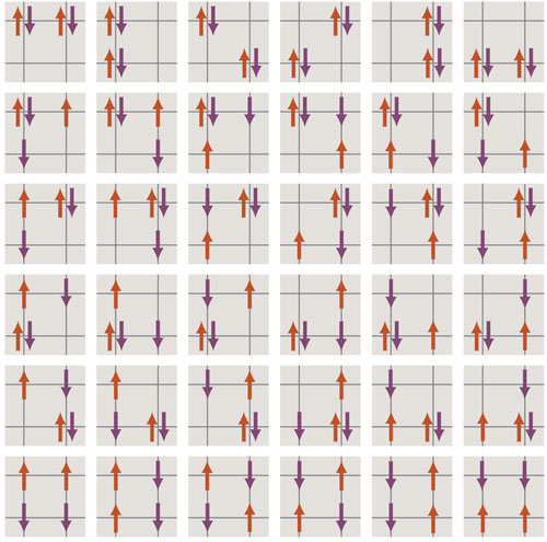
With these facts in hand, we can get a rough vision of the Hubbard model in action. Suppose the lattice is two-dimensional, like a sheet of graph paper. Some of the lattice points are occupied by electrons; some of those electrons are spin-up and the rest are spin-down. Thus a site can have any of four occupation states: no electrons, one up electron, one down electron or a pair of electrons with opposite spins. An electron can hop to any neighboring site, provided the move is allowed by the exclusion principle.

There’s one more essential element to introduce: the energy of the electrons. The exclusion principle requires that electrons with the same spin have distinct energies, which means there must be a ladder of available energy levels. If all the electrons have the same spin, they will necessarily fill all the rungs of the ladder from bottom to top. However, if half the electrons are spin-up and half are spin-down, they can be packed two to a rung, lowering the average energy level. This sharing of levels means that configurations with mixed spins can be energetically favorable.

On the other hand, the presence of both up and down spins also allows pairs of electrons to occupy the same lattice site, which incurs an energy penalty because of their mutual repulsion. For each doubly occupied site, the overall energy of the system increases by an amount designated U. Thus there is a subtle competition between the cost of populating higher levels of the energy ladder and the cost of overcoming electromagnetic repulsion.

What happens when we push the Start button and let the electrons hop around on the lattice? In general, this is a very hard question, but a few “corner cases”—where some parameter is set to an extreme value—offer clues. One such parameter is the number of electrons. For a lattice of N sites, this number must lie between zero and 2N. Nothing much happens with zero electrons, of course, and it turns out the same is true with 2N electrons: All sites are filled with paired electrons, and none of the electrons can move.

Another parameter is U, the energy of electrostatic repulsion for electrons at the same lattice site. If U is zero (no repulsion at all), the spin-up and the spin-down electrons form two independent populations, each of which drifts through the lattice oblivious of the other’s existence. At the opposite extreme, if U is infinite, the repulsion is so great that no site ever holds more than one electron. In this circumstance electrons can move only when there is an adjacent vacant site; if the lattice is half full (N electrons, with no vacancies), the configuration is frozen solid.

Still another parameter, whose role I have neglected so far, is temperature. At a temperature of absolute zero, the Hubbard model is compelled to adopt the configuration of lowest possible energy—the ground state. Thermal agitation at higher temperatures allows the system to escape this fate. With warming, higher-energy states come within reach. At infinite temperature all possible configurations are equally likely, and energy differences between states cease to have any influence on the behavior of the system.

As a practical matter, interest focuses not on the extreme cases but on realistic values of the parameters. Physicists would most like to know what happens when the number of electrons is at or near half-filling (one electron per site) and when the repulsion parameter U is greater than zero but far from infinite. As for temperature, it is important to identify the ground state, but we would also like to know how the behavior of the system changes as it warms up from absolute zero.

An Electronic Mosh Pit

The Hubbard model was invented in the early 1960s by John Hubbard, a British physicist who died young in 1980. Martin Gutzwiller of IBM Research in Zurich devised a similar model at about the same time, and investigators in Japan were also thinking along the same lines.

There were two main motivations for the model—two phenomena in need of theoretical explanation. One aim was to understand the mechanism of ferromagnetism. There had certainly been progress in this direction since the time of Lenz and Ising; in particular, a model developed in the 1930s by Werner Heisenberg adopted the simple lattice of the Ising model but gave a more realistic quantum-mechanical account of how adjacent spins interact. Still, the Heisenberg model left the spins stationary on the lattice, whereas the electrons that give rise to ferromagnetism in elements such as iron and nickel are not strictly localized; they can migrate from atom to atom. The Hubbard model allowed for such motion.

The second question addressed by the Hubbard model concerned electrical conductivity—or the lack of it—in certain crystalline compounds such as copper oxide (CuO). In most insulators, all the electrons are tightly bound to atoms or molecules, leaving no mobile electrons to carry a current. In the case of CuO, the theory of solids suggested there should be an ample supply of conduction electrons, and yet the material is an insulator. In 1937 Nevill Mott proposed an explanation: CuO fails to conduct not for lack of electrons but because the electrons can’t get out of each other’s way. The conduction band of this substance is like a crowded dance floor, where everyone desperately wants to keep moving but there are no vacant spaces to move into. By the 1960s the Hubbard model offered hope of better understanding such Mott insulators.

In recent years, the struggle to understand new high-temperature superconducting materials has intensified interest in the Hubbard model. The superconductors are layered materials whose components include copper oxides. Philip W. Anderson of Princeton University has argued that a two-dimensional Hubbard model can account for the transition to superconductivity in the copper oxide layers. This view remains controversial; on the other hand, the mere possibility of solving the puzzle of cuprate superconductivity has led to a frenzy of work on the Hubbard model and its variations.

The Electron Do-Si-Do

The only exact solution of a Hubbard model applies to the one-dimensional case, where the electrons move back and forth along a line of sites. In 1968 Elliott H. Lieb, now of Princeton University, and F. Y. Wu of Northeastern University studied the behavior of the one-dimensional system at half-filling (N electrons on N sites) as the value of U is varied. At large U (strong repulsion), the system is an insulator; Lieb and Wu proved there is no transition to a conducting state at any U greater than zero. They also showed that the ground state of the linear model is not ferromagnetic but antiferromagnetic: The lowest-energy configuration is one in which alternate spins point in opposite directions.

Lieb and Wu got their results by exploiting special properties of one-dimensional systems. In particular, there is no way for one electron to exchange places with another electron except by performing a kind of do-si-do, in which the two particles simultaneously occupy the same site. Because of the Pauli principle, two electrons in the same spin state can never change their ordering along the line. These constraints, which simplify the analysis, do not hold in higher dimensions.

Forty years later, the work of Lieb and Wu remains the only rigorous solution to a Hubbard model. But there are lots of less-than-rigorous hints and clues from approximation methods and from computer simulations.

It is widely believed that the two- and three-dimensional models also have an antiferromagnetic ground state—a checkerboard of alternating up and down spins—when the lattice is half-filled. An informal argument in support of this view points out that a fully magnetized system has only one possible configuration, since none of the electrons can move; in the antiferromagnet, adjacent electrons with opposite spins can swap places through the do-si-do mechanism. Thus there are many equivalent configurations for an antiferromagnet, which lowers the overall energy.

Can a Hubbard model ever favor ferromagnetism? Yes. In the 1960s Yosuke Nagaoka of Kyoto University discovered a ferromagnetic phase that appears when two conditions are satisfied: the repulsive interaction U is very strong, and the number of electrons is just short of half-filled. A single vacancy (that is, N–1 electrons on N sites) is enough to make the difference! Ferromagnetism also emerges spontaneously in Hubbard-like models in which the electrons can hop farther than the nearest-neighbor sites. One such scheme was described in 1995 by Hal Tasaki of Gakushuin University in Japan.

What’s intriguing about both ferromagnetism and antiferromagnetism in Hubbard systems is that the orderly configurations arise even though the model includes no direct interactions between pairs of electrons that would tend to align the spins either parallel or antiparallel. This is quite different from the Ising model, where parallel spins benefit from an energy bonus. In the Hubbard model—and surely in real solids as well—long-range order comes from subtler correlations within the entire population of electrons.

Why Is Hubbard So Hard?

The long-range correlations that make the Hubbard model interesting also make it hard to solve. One aspect of this difficulty is the vast number of possible configurations. On a 20-site lattice, 10 spin-up electrons and 10 spin-down electrons can be arranged in more than 34 billion ways. Yet this combinatorial explosion is not the main impediment to working out the fate of a Hubbard system. Other models in statistical mechanics also have huge numbers of configurations, yet various methods of analysis or simulation yield accurate results in those cases.

The real source of difficulty in the Hubbard model is the quantum entanglement of all the electrons. In the Ising model we can flip a spin at one site and consider only the local consequences—the change in energy between that spin and its immediate neighbors. In the quantum treatment of the Hubbard model, shifting an electron from one site to another can alter the state of the system arbitrarily far away. (The quantum state is defined by a wave function that can be smeared out over the entire lattice.)

Following the evolution of the Hubbard system by means of exact computations is all but unthinkable except for the tiniest models. It involves working with a matrix of size M × M, where M is the number of possible configurations. Michael Creutz of Brookhaven National Laboratory has experimented with a few such computations, reducing the storage requirement by tricks such as encoding lattice configurations in the bits of an integer. He was able to study a one-dimensional lattice of six sites—essentially a benzene molecule—with a matrix of 400 × 400 elements. But he points out that a two-dimensional lattice of just 16 sites would have some 165,636,900 configurations.

The problems of working with these large matrices go beyond mere demands for storage space and computing time. It turns out that the matrix is often “ill conditioned”; when the algorithm calls for computing a small difference between two large numbers, all accuracy is lost and the matrix fills with useless numerical noise.

But I should not leave the impression that computation is a lost cause in the Hubbard model. On the contrary, it has been the main source of insight over the past 40 years. No one algorithm has conquered the problem overall, but a toolkit of specialized methods have tamed many corners of it. For example, there are algorithms that perform well for values of N near half-filling, and other methods that work best when U is large. One strategy, pioneered by a group headquartered at the University of California, Santa Barbara, takes the counterintuitive step of replacing a large matrix with an even larger one—but the replacement matrix ameliorates the problem of lost numerical accuracy.

Back to the Lab Bench

The newest trick in the long struggle to master the Hubbard model is the idea of setting up experimental apparatus to mimic the model’s lattice and its population of electrons. Standing in for the electrons in these experiments are atoms of an ultracold gas—so cold, and therefore so sluggish, that the atoms can be trapped by the feeble electromagnetic field of a beam of light. Three such beams crossing at right angles create a sort of three-dimensional egg carton, with periodic wells where the cold atoms tend to accumulate. The atoms chosen for the experiment are members of the same quantum-mechanical class as electrons (known as fermions), and so they are subject to the same quantum rules as the electrons in a solid; in particular, no two atoms in the same spin state can occupy the same site in the optical lattice. Furthermore, two atoms of differing spin that land on the same site experience a short-range repulsion, just as electrons do. Thus the stage is set for a full simulation of the Hubbard model. The optical lattice is typically a few millimeters across, and it holds tens of thousands of atoms.

Of course it’s easy to talk about the principles of such an experiment; making it happen in the laboratory is harder—indeed, heroic. But in recent months three groups have reported successful results of such experiments. Two of those groups have found evidence of a Mott-insulator phase in the confined atoms. (The groups are led by Immanuel Bloch of Johannes Gutenberg University in Mainz, Germany, and by Robert Jördens and Niels Strohmaier of the Swiss Federal Institute of Technology in Zurich.) The third group, led by Gyu-Boong Jo of MIT, has seen signs of ferromagnetic order in a gas of cold atoms.

There is something deliciously involuted about this turn of events: an experiment that illuminates a model that explicates an experiment. One interpretation is that the assembly of lasers and cryogenic atoms and other apparatus is acting as a special-purpose quantum computer, which can efficiently solve problems that would require exponentially greater effort on a classical computer.

This audacious approach to doing science—harnessing physics to do the work of mathematics and computation—surely has great promise; and yet I have a nagging reservation. As I said at the beginning of this essay, a mathematical model is an aid to understanding, not just an engine for producing answers. According to this view, the aim of the Hubbard model is not so much to determine whether certain kinds of solids have ferromagnetic order or Mott transitions or superconducting phases. What the model offers is hope of understanding where those traits come from—how the basic ingredients of the model combine to yield emergent properties. The cold-atom experiments seem less effective as aids to understanding: Even when they yield the right answer, we may not easily see why it’s right. The experiments get their power from the same quantum mysteries they seek to explain.

The same complaint has often been made about ordinary computer simulations and about computer-aided proofs in mathematics. If the computer is just a black box, and we cannot follow along step by step from premise to conclusion, how can we pretend to understand the result? But these doubts about the legitimacy of computer-aided science seem to be fading, chased away by the spread of algorithmic thinking. Perhaps now we need to wait for a wider embrace of quantum thinking.

To my readers

After the publication of this column (my 97th since 1993), I will be taking a one-year sabbatical leave from the Computing Science department. Although I have a long list of topics for columns that I’m still eager to learn about and write about, I also have other projects I’ve deferred too long. After a year’s respite from bimonthly deadlines, I look forward to returning to this splendid soapbox in 2011. In the meantime, this space will be filled with fresh voices and viewpoints. For those who wish to follow my own ongoing adventures, I expect to continue posting occasional essays at bit-player.org.—Brian Hayes

©Brian Hayes