American Scientist

In the winter of 1917 Lewis Fry Richardson was driving an ambulance for a French infantry division on the Western Front. At the same time, in spare moments behind the lines, he was completing a vast project of mathematical calculations. He had set out to compute the weather, to predict the temperature, the winds and the barometric pressure from first principles of physics. It would have been an ambitious undertaking in the best of circumstances—in a quiet study with a long oak table for spreading out the paperwork. Richardson did it in the middle of a war that was, among its other distinctions, the muddiest in human history. "My office," he wrote, "was a heap of hay in a cold rest billet."

Richardson's goal was to follow the development of the weather for a six-hour interval in a small area of central Europe. Even a forecast of this limited scope called for a calculation of daunting complexity. Needless to say, he had no electronic computer to do the arithmetic for him. He worked with pencil and paper, as well as a slide rule and a table of logarithms. To guard against careless mistakes he did everything twice.

The outcome was not a conspicuous success. The actual weather changed little over the period of the forecast, but Richardson's equations had the barometer rising fast enough to make your ears pop. The calculation was a brilliant piece of work nonetheless. Although he failed to predict the weather, he predicted the future of weather prediction. The forecast you now see on the six o'clock news is based on simulations remarkably like Richardson's (including the occasional error).

What went wrong with that first-ever numerical forecast? Many commentators have suggested explanations, starting with Richardson himself. A new analysis takes a direct approach to understanding the source of the problem. Peter Lynch of Met Éireann, the Irish Meteorological Service, has carefully reconstructed and replicated the entire calculation—everything but the heap of hay in the rest billet. He has been able to reproduce Richardson's error, and even to correct it.

Off the Tenure Track

Before diving into the differential equations, it is worthwhile pausing to look back over Lewis Fry Richardson's life and career, which were no less strange and wonderful than his scientific work. He came from a prosperous family in Newcastle upon Tyne, the industrial port in the far north of England. They were Quakers, and Lewis was sent to Bootham, a distinguished Quaker boarding school, where his interests in science and natural history were cultivated by J. Edmund Clark, a prominent member of the Royal Meteorological Society. "Another master," Richardson later wrote, "left me with the conviction that science ought to be subordinate to morals."

At Cambridge, Richardson's mentor was J. J. Thomson, the Cavendish professor of physics (and the discoverer of the electron). Richardson took first-class honors in natural sciences. Later he sought a fellowship at King's College, but he was passed over. There followed a decade of short-term, low-ranking jobs in out-of-the-way places, like the succession of postdoc appointments so many graduates face today. In the end Richardson never did hold a chair at any of the major British universities.

In 1913 he became superintendent of the Eskdalemuir Observatory in the Scottish Southern Uplands. Talk about out-of-the-way places! This small institution, run by the Meteorological Office, had been founded to measure variations in the earth's magnetic field, and it was deliberately put as far as possible from railroads and power lines. Richardson described it as a place of "bleak and humid solitude," but this was probably not a complaint; when he was once asked if he had any hobbies, his answer was "solitude."

In any event, the solitude was soon interrupted. "In August 1914," Richardson wrote later, "I was torn between an intense curiosity to see war at close quarters and an intense objection to killing people, both mixed with ideas of public duty and doubt as to whether I could endure danger." He requested a leave of absence but was refused. In 1916 he resigned his post and joined the Friends' Ambulance Unit.

After the war, Richardson returned to the Meteorological Office, working at the Benson research station near Oxford, but that job also ended prematurely. In 1920 the Meteorological Office was put under military administration, and Richardson felt compelled to resign again. After that, he never got back on the tenure track.

Some biographers emphasize the price that Richardson paid for his convictions. According to family members, his pacifist principles cost him a university appointment. Family memoirs also describe an anguished moment when he destroyed his research on atmospheric turbulence because it was attracting the attention of "the 'poison gas' experts." On the other hand, it would be misleading to portray Richardson as an outcast from the scientific establishment. He was elected a Fellow of the Royal Society; he served as secretary of the Royal Meteorological Society; he had well over 100 scholarly publications (recently collected in two fat volumes by Cambridge University Press). Today there is a Richardson Institute for Peace Studies and Conflict Resolution, and one of the dimensionless numbers of fluid mechanics is called the Richardson number.

Whether for reasons of conscience or pure predilection, Richardson did turn away from work in meteorology after the mid-1920s. He took a degree in psychology (at age 48), and then for the last 15 years of his life focused on the study of war and its prevention. He took a mathematical approach to these problems as well. For most people, the idea that mathematics might be the key to world peace seems naive and implausible, but maybe we shouldn't be too quick to give up on it. In Richardson's day, mathematics also looked like an outlandishly unsuitable tool for weather forecasting.

Checkerboard Europe

Richardson's forecast was actually a hindcast: He was "predicting" events that had taken place years before. His initial data described the state of the atmosphere over Germany and neighboring countries at 7:00 a.m. (Greenwich time) on May 20, 1910. His goal was to model the weather in this region over a span of six hours. He chose this particular time and place not because the weather was in any way unusual that Friday morning but rather because unusually good data were available. May 20, 1910, was one of a series of days on which weather observations were collected from coordinated balloon ascents all over Europe. The results had been tabulated and analyzed by the Norwegian meteorologist Vilhelm Bjerknes.

The observing sites for the Bjerknes project were scattered irregularly across the map of Europe, and so Richardson had to interpolate to produce a uniform grid of data points. The grid he chose was a checkerboard, with squares roughly 200 kilometers on a side. A pattern of 25 squares covered a diamond-shaped region extending from Denmark to Italy and from the English Channel to Poland. Vertically, he sliced the atmosphere into five layers, with boundaries at altitudes of roughly 2, 4, 7 and 12 kilometers. (The heights were chosen so that each stratum had about the same mass of air.) Thus the model divided the volume being studied into 125 compartments.

The pattern of squares laid out on the landscape was described as a checkerboard rather than merely a grid because different quantities were computed in the alternating black and white squares. In one set of squares (called P cells) Richardson recorded the barometric pressure in each of the five altitude layers, and also moisture amounts and the stratospheric temperature. In the other squares (M cells) he calculated the momentum of the atmosphere—that is, the wind speed and direction multiplied by the mass of the air.

It's not hard to see in a qualitative way how these variables would enter into a model of the atmosphere's dynamics. In particular, winds and barometric pressures have an obvious interconnection. Pressure is the force that drives the winds; air flows from place to place in response to differences in pressure. At the same time, the convergence or divergence of winds alters the pressure in a region, as air is either blown in or sucked out. A similar linkage connects pressure with temperature, since heat is generated when air is compressed. The model has to track all these relationships (and others) from moment to moment. Given initial values of all the variables at time t₀, the model calculates the values at a later time t₁; then these t₁ values form the basis of a new calculation at time t₂, and so on.

The most important quantities to keep track of in Richardson's model turned out to be barometric pressure and three components of momentum (along north-south, east-west and up-down axes). All of these quantities vary from place to place and from moment to moment; in other words, they are functions of latitude, longitude, height and time. There are also crucial dependencies among them. For example, one of Richardson's equations states that the rate of change in the east-west component of momentum depends on the pressure gradient along the same axis. This relation is unsurprising; it says that air goes where you push it. But the full atmospheric equations of motion are more complicated. In addition to the pressure-gradient term, they also includes a term representing the Coriolis force, by which the earth's rotation twists the winds and thereby couples east-west and north-south velocities.

Vertical motions in the atmosphere are even more problematic. No vertical winds were included among the initial data. To calculate them, Richardson relied on a simple ground truth: The earth is solid, and therefore impervious to wind. It follows that if horizontal winds are converging in some ground-level cell of the model atmosphere, then air must be flowing upward out of that cell. By the same principle, divergent winds at ground level must be balanced by air sinking into the cell from above.

Leapfrog Integration

In general, the system of differential equations describing the behavior of the atmosphere cannot be solved exactly. Bjerknes advocated a graphical method of finding approximate solutions, but Richardson favored numerical techniques. Specifically, he adopted a finite-difference method, replacing continuously varying fields with changes calculated over discrete intervals. For example, consider the calculation of the winds in a given M cell. In the discrete model the change in the east-west component of the wind depends on the difference between the pressures in the P cells to the east and the west; in the same way the north-south component is calculated from the difference in pressure values to the north and south.

Boundary conditions present an annoying complication. If the winds in an M cell depend on the four surrounding P cells, what happens at the edge of the array, where some of the P cells do not exist? The ideal solution would be to cover the entire globe, so there are no edges, but that option was beyond Richardson's reach. Instead he ducked the question by making his prediction only for two squares (one M cell and one P cell) in the middle of his diamond-shaped array. Thus he made use of the initial values in the boundary cells but did not try to calculate new values there.

Time as well as space is discrete in Richardson's scheme. He chose a basic time unit of Δt=3 hours. He also employed a "leapfrog" method of numerical integration, where events at time t+1 depend on the state of the system both at the present time t and at the previous moment t–1. But the leapfrog process hardly got started in Richardson's calculation. He carried out only a single step of the integration, computing the "initial tendencies"—the rates of change in pressure, momentum, etc.—and used these tendencies to compute the changes in the weather over a period of 2Δt, or six hours, centered on 7 a.m.

Here are the results, as Richardson reported them in his book Weather Prediction by Numerical Process. In the central M cell, which covered the area surrounding Nurenberg and Weimar, the surface wind freshened somewhat over the six hours of the forecast, while the stratospheric winds increased more than tenfold. An even more dramatic change was seen in the P cell to the south, over Munich. According to the model, barometric pressure in the lowest stratum rose by 145 millibars to 1,108 millibars. If this surface pressure had been correct, it would have been a world record; the actual barometric reading was nearly steady on that day.

The Answer Is Blowin' in the Wind

What went wrong? The prime suspect in a case like this one is usually numerical instability. When the result of one step serves as the input for the next step, small errors can multiply and grow explosively. There is a rule for avoiding such a catastrophic loss of accuracy: The time step must be kept shorter than the time needed for information to propagate through the model—in this case between observing stations spaced every 200 kilometers. According to this criterion, Δt in Richardson's model should have been no more than about 30 minutes. Richardson can hardly be blamed for breaking this rule—the limit on Δt was not discovered until a decade later (by Richard Courant, Kurt Otto Friedrichs and Hans Lewy)—but the model is clearly in violation all the same.

The Courant-Friedrichs-Lewy condition has been cited as a possible cause of failure by several commentators on Richardson's work, including Sydney Chapman in the preface to a reprinting of Weather Prediction by Numerical Process. Nevertheless, numerical instability cannot be the source of the problem. Errors grow exponentially when the finite-difference procedure is iterated, with the output of each stage becoming the input to the next stage. Richardson stopped calculating after one step. If he had kept going, instability would doubtless have appeared, but it can't explain a large error in the initial tendencies.

Another possible culprit is the phenomenon called deterministic chaos, which Edward N. Lorenz described 35 years ago, also in the context of weather prediction. Lorenzian chaos is superficially similar to numerical instability, but a chaotic system remains unpredictable even if each step of the calculation is performed with perfect precision. The slightest change in the initial conditions is enough to produce a divergent result. There is no question that Richardson's calculation would be subject to this problem if it were continued long enough, but again chaos can't explain a failure in the first step.

The real cause of Richardson's forecasting error was identified by Richardson himself. At the end of his table of results, he wrote: "It is claimed that the above form a fairly correct deduction from a somewhat unnatural initial distribution." In other words, the problem lay not in the algorithm but in the input data. A close look at the data confirms this diagnosis and also shows clearly why weather prediction is such a hard problem.

The main troublespot is the part of the calculation where pressure is determined from the convergence (or divergence) of winds. Along each horizontal axis, the wind convergence is calculated as the small difference between two large numbers. Under these circumstances, even slight errors in the initial wind data can cause large variations in the computed convergence. For example, suppose the true east-west winds on either side of a P cell have magnitudes of 101 and 99 (in some appropriate system of units). Then the east-west convergence is equal to 2. If the measurement of either wind is off by just 1 percent, however, the convergence will change by 50 percent or 100 percent. This disastrous error in convergence will be reflected in the predicted barometric pressure.

Another property of the atmosphere compounds the sensitivity to measurement errors. If low-level winds in a region are converging, upper-level winds over the same area are usually diverging. This state of balance tends to reduce the effect that convergence or divergence would have on barometric pressure, but again the balance is easily upset by measurement errors.

And just as errors in wind measurement degrade the prediction of pressure, so also pressure errors confound wind predictions. Here too the culprit is the subtraction of two nearly equal quantities—the pressure-gradient term and the Coriolis term in the atmospheric equations of motion. Because the terms generally have about the same magnitude, small errors in observations yield large changes in predicted wind.

Richardson recognized these mechanisms and suggested smoothing the initial data as a possible remedy. Lynch points out that the problem goes deeper. To maintain the overall state of balance in the atmosphere, smoothing either the winds or the pressures is not enough; the two sets of observations have to be made mutually consistent.

The Orchestra of Slide-Rules

For his reconstruction of the Richardson experiment, Lynch went back to the original weather charts for May 20, 1910, and redid the interpolation process. He found only one likely error in Richardson's initial data—a suspiciously low pressure over Strasbourg. Data values elsewhere were in good agreement.

Although Lynch set out to create a faithful reproduction of Richardson's model, he did not do the arithmetic with pencil and paper; the model was implemented as a computer program. But even though computing power was not a limiting resource, Lynch decided to simplify the model in some respects. A curiosity of Richardson's work is that he included certain physical and even biological phenomena that now seem marginal. He was a shrewd numerical analyst, and he must have been able to estimate the importance of each term in his equations; nevertheless, he invested much effort in modeling factors that could not possibly have much effect on the overall outcome. For example, he calculated the temperature of the soil at various levels and the effects of vegetation on moisture in the atmosphere. These influences might be barely detectable in a high-precision weather model, but it was premature to build them into this first crude experiment. Lynch neglects these factors, and indeed drops all consideration of water in the atmosphere.

The results of Lynch's replica computation are quite close to those of the original. The surface-level rise in pressure was 145.1 millibars according to Richardson, and 145.4 according to Lynch. Predicted winds do not match quite as closely, but the average discrepancy is only about 13 percent.

Having reproduced Richardson's faulty calculation, Lynch then went on to try correcting it. The problem of initial observations that are not in harmony persists in weather prediction today, but digital filtering techniques have been devised to reconcile the wind and pressure fields. Lynch applied one of these filtering methods, which essentially runs the model both forward and backward from the starting point to generate a consistent set of values. With the filtered data, and with a smaller Δt to ensure numerical stability, all results were physically plausible and in reasonably good agreement with observations. Richardson came that close to getting it right.

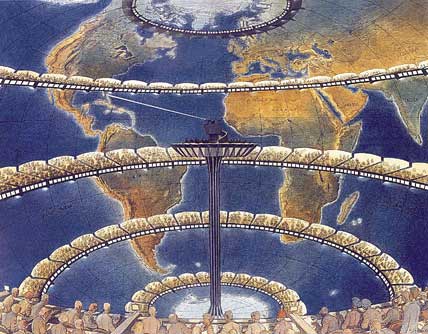
Richardson ended his book with a daydream about the future of numerical weather prediction. He estimated that it would take 64,000 computers (and by "computers" he meant people) to keep up with all the world's weather. The work might be done in a great spherical hall. "The walls of this chamber are painted to form a map of the globe. The ceiling represents the north polar regions, England is in the gallery, the tropics in the upper circle, Australia on the dress circle and the antarctic in the pit. A myriad of computers are at work upon the weather of the part of the map where each sits.... From the floor of the pit a tall pillar rises to half the height of the hall. It carries a large pulpit on its top. In this sits the man in charge of the whole theatre.... One of his duties is to maintain a uniform speed of progress in all parts of the globe. In this respect he is like the conductor of an orchestra in which the instruments are slide-rules and calculating machines. But instead of waving a baton he turns a beam of rosy light upon any region that is running ahead of the rest, and a beam of blue light upon those who are behindhand."

Lynch and others have pointed out that the estimate of 64,000 computers was a serious undercount. Even by Richardson's own criteria, the number probably should have been 200,000, and a modern estimate would be much larger still. Indeed, if we were to try to do by hand labor all the computing that is nowadays dedicated to weather prediction, the entire human population could not keep up. Thus Richardson's orchestra of slide-rules was never a realistic possibility. Practical forecasting by numerical methods could not have begun much sooner than it did, with the work of Jule Charney and John von Neumann around 1950.

Nevertheless, Lynch concludes his article with a wistful consideration of what might have been, if Richardson's early forecast had not gone awry. "Let us suppose that Richardson had applied some filter, however crude, to his initial data. His results might well have been realistic, and his method would surely have been given the attention which it certainly deserved." I would not disagree, and yet at the same time I find that what is most interesting about the forecast is its failure, and what is most admirable about Richardson is his determination to publish it anyway. The failure of the experiment even made it worth repeating.

© Brian Hayes