American Scientist

Forty years ago this spring, a little book titled The Limits to Growth landed with a big thump. The authors reported on an exercise in computer modeling, which they grandly described as “Phase One of the Project on the Predicament of Mankind.” According to the model, the human predicament was bleak, with less than a century to go before civilization would crumple under the burdens of overpopulation, famine, resource depletion and pollution. As a young journalist I was fascinated by this apocalyptic vision. I was also intrigued by the remarkable idea that computation might be a useful tool for understanding the human predicament.

In 1972 I had no way to explore the workings of the Limits model for myself. Twenty years later, though, with a desktop computer and ready-to-run modeling software, I was able to twiddle the model’s various knobs and observe the effects on the outcome. I wrote about that experience in 1993, in the first column published in these pages under the rubric “Computing Science.”

Recently I have turned to the Limits model yet again, this time delving into details of its implementation—the 150 equations that govern the evolution of the simulated world. Closer examination of the model’s structure has not increased my confidence in its predictive power. On the other hand, the hope that computation might have something to tell us about the fate of the planet remains very much alive. We don’t have an abundance of better tools for seeing into the future. An interesting challenge is to clarify what distinguishes the computational methodology of The Limits to Growth from other models that policymakers take more seriously, such as the climate models that now underlie much of the discussion of global warming.

System Dynamics

The Limits to Growth lists four authors (Donella H. Meadows, Dennis L. Meadows, Jørgen Randers and William W. Behrens III) as well as a project team with 17 members, but the principal architect of the modeling scheme presented in the book is not among these individuals. He is Jay W. Forrester, who arrived at the Massachusetts Institute of Technology in 1939 as a graduate student in electrical engineering and who is there still, almost 75 years later, as professor emeritus. Forrester’s early work was on automatic control and servomechanisms. Later he built the largest digital computer of its time and invented magnetic core random-access memory, which dominated the industry for 20 years.

In 1956 Forrester moved across campus to the Sloan School of Management, where he began applying ideas from control engineering—particularly the idea of feedback—to problems of business. For example, he explained cyclic waves of hiring and layoffs as an “overshoot” phenomenon, where managers responded too late or too vigorously to changes in sales or inventory.

Feedback loops and the risk of overshooting became recurrent themes in a methodology that Forrester named system dynamics. He was soon extending the scope of the technique: His book Industrial Dynamics, on the management of companies, was followed by Urban Dynamics, on the management of cities.

In 1970 Forrester attended a meeting of the Club of Rome, a loosely organized “invisible college” on the lookout for novel approaches to social and environmental problems. On the flight home he sketched a system dynamics model of the world economy and ecosystem. A few weeks later he had a working prototype, which came to be known as World2. The Club of Rome proposed to sponsor this work, but Forrester chose to continue his project independently; a year later he published his findings in World Dynamics. Meanwhile, his colleague and former student Dennis Meadows assembled a team for the Club of Rome project. Their version of the model is World3.

Vats and Valves

A diagram of a system dynamics model could well be mistaken for the schematic layout of an oil refinery. Various tanks or vats are connected by pipes; flows through the pipes are regulated by valves; the valves are controlled by signals that derive from the state of reservoirs or flows elsewhere in the model.

The World3 model has five main sectors: population, agriculture, industry, resources and pollution. In the population sector, the quantities held in the vats and flowing through the pipes are people; the valves controlling the flows represent birth rates, death rates and the process of maturation that carries people from one age category to the next. The agricultural sector has stocks of arable land, which are augmented when new land is cultivated and diminished when farmland is lost to erosion or urban development. The main stock for industry is capital, which is measured in dollars but really represents factories or other productive facilities. The level of capital is determined by the balance of inflow from investment and outflow to depreciation.

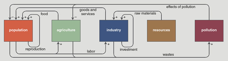
If you examine a small region of the plumbing diagram in isolation, you can often figure out how that subsystem will behave. For example, the resources sector of the model includes only nonrenewable resources such as ores and fossil fuels, and so the level of this stock can never rise. The rate of resource outflow is governed by the total population and the per capita level of resource consumption.

Looking at the entire Rube Goldberg diagram—which won’t fit comfortably on a page smaller than a newspaper broadsheet—there’s no hope of understanding all the interactions at a glance. This is the reason for turning the conceptual model into a computer simulation: The computer can keep track of the levels and flows as the system evolves.

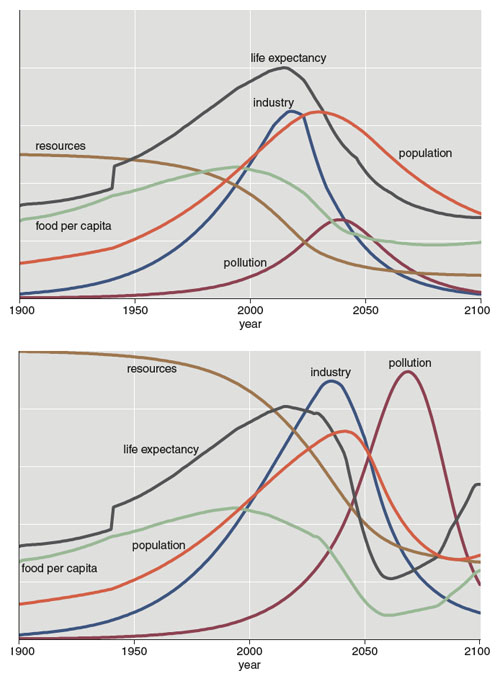
The World3 simulation covers the period from 1900 to 2100. In the standard run, using default values for all parameters, nonrenewable resources are exhausted by the middle of the 21st century, causing steep declines in industry, food and population. Adjusting the initial conditions to double the available resources alters the outcome, but not for the better: Higher industrial output leads to runaway pollution, which chokes off growth—and even life—a few decades later. The persistent shape of the model’s trajectory is overshoot followed by collapse.

World3 War

The Limits to Growth appeared at a moment of acute environmental foreboding. The previous decade had seen the publication of Rachel Carson’s Silent Spring, Garrett Hardin’s “Tragedy of the Commons” essay, Paul R. Ehrlich’s The Population Bomb and Barry Commoner’s The Closing Circle. This was the era when we began to refer to our planet as Spaceship Earth, and when Walt Kelly’s Pogo declared “We have met the enemy and he is us.” There was a receptive audience awaiting The Limits to Growth. The book has sold 10 million copies.

But if Limits has had a broad and sympathetic readership, it has also had vociferous critics. The most carefully argued rebuttal came from a group at the University of Sussex in England; their critique, Models of Doom, is longer than the book it evaluates. The economist William D. Nordhaus wrote a blistering review; the mathematician David Berlinski was snide and mocking. Vaclav Smil later dismissed the whole enterprise as “an exercise in misinformation and obfuscation.”

One complaint lodged against the World3 model is superfluous complication. If the intent is merely to show that exponential growth cannot continue forever, there’s no need for elaborate computing machinery. The model also stands accused of the opposite sin—oversimplification—in its wholesale aggregation of variables. In the resource sector, for example, the model lumps together all the raw materials of industrial civilization—coal and oil, iron and aluminum, diamonds and building stone—to form one generic substance measured in abstract “resource units.” Pollution is handled the same way, with a single variable encompassing everything from pesticides to nuclear reactor wastes. Quantities such as food per capita are global averages, with no way of expressing disparities of distribution. (A later Club of Rome model, written by Mihajlo Mesarovic and Eduard Pestel, did allow for regional differences.)

Still another line of criticism focuses on the inputs to the model—the initial conditions (such as the total stock of nonrenewable resources) and the numerical constants that determine the strength of interactions (for instance, the effect of pollution on agriculture). The Limits team made an effort to pin down these numbers, but huge uncertainties remain. There is no statistical analysis of these errors.

Both Forrester and the Limits group have responded to these objections, matching the vehemence—and occasionally the condescending scorn—of their critics. They stand by their models. When updated versions of the Limits book were published in 1992 and 2004, the authors reiterated their original conclusions and made only subtle changes to the model.

World3 now seems to be undergoing a revival. In 2009 Charles A. S. Hall and John W. Day, Jr., writing in American Scientist, defended the soundness of the model, particularly as it applies to energy resources. Graham Turner has compared predictions with data for 1970–2000 and reports a close match. Ugo Bardi, an Italian chemist, has recently issued a manifesto calling for the rehabilitation of The Limits to Growth.

The Dusty Deck

After 40 years of intense scrutiny, further probing of the World3 model is unlikely to yield big surprises. Nevertheless, nagged by a feeling that I still didn’t really understand the model, I decided to take it apart and put it together again.

When I wrote about Limits in 1993, I worked with a simulation package called Stella II, which offers a snazzy interface: You build a model by dragging icons of vats and valves across the screen. For my studies of World3 I was spared even that labor because a prebuilt version of the model came with the software. Stella II is still available, and so are competing products such as Modelica, Simgua and Vensim. These are impressive programs, recommended for serious work with system dynamics models. My aim, however, was not just to run or test the World3 model but to see how the parts fit together. I wanted to bake my cake from scratch, not from the Betty Crocker box.

The original World3 model was written in a language called DYNAMO, developed in the early 1960s by Phyllis Fox and Alexander Pugh for the Forrester group at MIT. The DYNAMO source code for the World3 model was published in Dynamics of Growth in a Finite World, a thick technical annex to The Limits to Growth. As a way of digesting the DYNAMO program, I decided to make a line-by-line translation into JavaScript, the scripting language built into Web browsers. (The result of this exercise is at http://bit-player.org/limits.)

DYNAMO comes from the Fortran era, when programs were fed to the machine on punch cards, and variables had names like “FIALD” (which stands for “Fraction of Inputs Allocated to Land Development”). Beyond these musty lexical conventions, however, lies an interesting programming language, little known outside the system dynamics community. It is mainly declarative rather than procedural. A program is not a sequence of commands but a list of “equations” (really assignment statements) that specify relationships of variables. The sequencing is handled behind the scenes by the DYNAMO compiler.

The World3 program consists of about 150 equations. The vats and valves of the plumbing diagram correspond to “level equations” and “rate equations,” respectively. A level equation calculates a new value for the level in a vat based on the level at an earlier moment and on the rates of inflow and outflow. The calculation is an integration, which would be represented as follows in DYNAMO:

V.K = V.J + DT * (IN.JK – OUT.JK)

Here V is a level variable, IN and OUT are rate variables, and DT is the integration interval, the unit of time in the simulation. The suffixes .J, .K and .JK are time markers: V.J and V.K represent the level of V at successive instants, and IN.JK is a rate of flow during the interval between time J and time K.

Just as levels depend on rates of inflow and outflow, the flow rates in turn can depend on levels. (Think of a bucket with a hole in the bottom: The rate of flow depends on the height of water in the bucket.) This kind of feedback loop is what gives the system the potential for interesting behavior, but from a computational point of view it is an awkward causal circularity. DYNAMO breaks the circle by updating levels and rates in alternation. The level at time t₀ determines the rate at t₁, which determines the level at t₂, and so on. Some conflicts are harder to resolve and require an explicit reordering of the equations, which DYNAMO handles automatically.

Supporting Actors

Levels and rates of flow are the principal actors in a system dynamics model, and they usually occupy the spotlight. But there is also a large supporting cast. Among the 150 equations of the World3 model there are just 12 level equations and 21 rate equations; all the rest are “auxiliary” equations of various kinds. In the course of reimplementing the model I learned that the tangled net of auxiliary equations is where most of the complexity—and perplexity—lies.

Level and rate equations are subject to strong constraints, rooted in physical conservation laws. The level of population, for example, can change only by adding births and subtracting deaths; the books of account must balance. The auxiliary equations are not constrained in this way. They represent flows of information rather than materials, and they can take almost any mathematical form. Furthermore, the information pathways of World3 form an intricately branching tree, so that tracing connections through the long chains of nodes is like playing “six degrees of separation.” One pathway between service capital and population is shown in the fourth illustration. The basic idea is simply that services include health services, which affect life expectancy and hence death rates; but it takes about a dozen steps to make the connection.

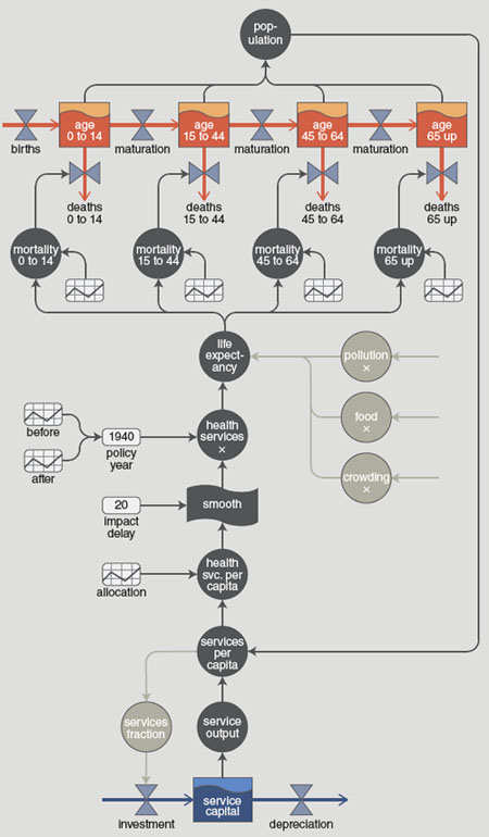
Many of the auxiliary equations have associated constants and coefficients, or even whole tables of constants. For example, the function relating service output per capita to health service allocation per capita is defined by a table of nine numeric values. More than 400 constants, coefficients, table entries and initial values appear in the model. They are not mathematically determined; they have to come from empirical knowledge of the real world. They represent a great many degrees of freedom in the construction of the model.

Interactions between auxiliary variables are a further source of complication—and mystification. As noted above, health services are assumed to have an effect on life expectancy. But life expectancy is also influenced by three other factors: nutrition, pollution and crowding. How are the four inputs to be combined? Mathematics offers an infinite spectrum of possibilities, but the most obvious choices are to add or multiply. The results can differ dramatically. Suppose the health services variable falls to zero: With an additive scheme, the variable would cease to have any effect on life expectancy, but with a multiplicative combining rule, life expectancy itself would be driven to zero. How does World3 do it? The rule is multiplicative, but with a clamping function that keeps life expectancy in the range from 20 to 80 years.

In bringing up this matter I don’t mean to suggest that one combining form is correct and another wrong; I merely want to call attention to how many subtle decisions are buried in the foundations of the model. And when I read through the program, I kept seeing opportunities for still more elaboration. For example, the demographic effects of health services might well vary depending on whether the services are for young people (vaccination) or older people (nursing homes). This refinement could certainly be incorporated into the model, along with many more, but would it be an improvement? Where do you stop?

Model Models

Very small models can yield surprisingly rich behavior. One example is the predator-prey model developed (independently) by Alfred J. Lotka and Vito Volterra early in the 20th century. With just two equations and four parameters this model explains cyclic fluctuations in the abundance of predators and their prey, such as wolves and moose. Feedback and overshooting lead to prolonged oscillations rather than a direct approach to equilibrium.

The simplicity of the Lotka-Volterra model is part of its appeal, yet we cannot insist that everything of interest in the world be crammed into no more than two equations. If you want to describe the whole of human society and the planetary ecosystem, you probably need a few more parameters.

In this context climate models offer a useful point of reference. General circulation models for the atmosphere and the oceans, along with related models of ice sheets and atmospheric chemistry, have several points of similarity with World3. At a conceptual level the structure is much the same: There are flows of air, water, heat and other entities, which the model must sum or integrate. The time scales are similar: In both cases we want to know what’s going to happen several decades out. And feedback loops are essential mechanisms in both kinds of models. (There are even historical connections. The use of general circulation models to study global climate change began in earnest at MIT circa 1970. The instigator was Carroll Wilson of the Sloan School of Management, who was also the person who got Forrester involved with the Club of Rome.)

These similarities are outweighed by differences. Where the Limits team had a casual attitude to data gathering practices—and outright hostility to statistical methods—the climate science community is passionate about collecting data, verifying its provenance and quantifying its uncertainty. General circulation models are not based on rough estimates or guesses but on decades of meticulously curated measurements—what Paul Edwards, in A Vast Machine , calls a “climate knowledge infrastructure.”

The organizational scale of the two undertakings differs by orders of magnitude. The World3 model was put together by a dozen people working in isolation for a year or two. Climate modeling is Big Science, with contributions from several hundred workers, organized in groups that both compete and collaborate, with institutional and governmental oversight, not to mention a great deal of public scrutiny. The process has been ongoing for 40 years.

Another difference is that climate models focus mainly on physical and chemical processes where the underlying science is generally well understood. We know a lot about the absorption and emission spectra of molecules in the atmosphere, and we know how a volume of air will respond to heating or to a change in pressure. The social and economic systems modeled in World3 do not have natural laws of the same predictive power. In this sense the climate problem is easier.

In another respect, however, the task of climate models is more demanding. Where World3 promises only to “illustrate the basic dynamic tendencies” of the system, climate models are expected to produce precise quantitative predictions, such as a 1 percent change in global average temperature.

Limits of Limits

After three immersions in The Limits to Growth, at intervals of 20 years, I feel entitled to state some opinions.

First, the book’s message is worth listening to. There are limits, and exponential growth is unsustainable. A society that measures well-being by the first derivative of GDP is asking for trouble. But I am more optimistic than the Limits authors are about our ability to deal with these issues before the world turns into the set of a Mad Max movie.

As for the mathematical model behind the book, I believe it is more a polemical tool than a scientific instrument. Forrester and the Limits group have frequently said that the graphs drawn by their computer programs should not be taken as predictions of the future, but only as indicating “dynamic tendencies” or “behavior modes.” But despite these disclaimers, Limits is full of blunt statements about the future: “If the present growth trends continue unchanged,... the limits to growth on this planet will be reached sometime in the next one hundred years.” And whether the models are supposed to be predictive or not, they are offered as an explicit guide to public policy. For example, in testimony before a congressional committee in the 1970s Forrester recommended curtailing investment in industrialization and food production as a way of slowing population growth.

It’s possible that Forrester was offering wise advice, and someday we’ll regret not taking it. But when a mathematical or scientific argument is brought forward to justify taking such a painful and troubling action, standards of rigor will surely be set very high.

In an unpublished paper on the testing of system dynamics models, Forrester and a student wrote: “The ultimate objective of validation is transferred confidence in a model’s usefulness as a basis for policy change.” That has yet to happen for World3.