Quasirandom Ramblings
By Brian Hayes
Random numbers have a peculiar power, even when they are only pseudo- or quasirandom
Random numbers have a peculiar power, even when they are only pseudo- or quasirandom

DOI: 10.1511/2011.91.282
In the early 1990s Spassimir Paskov, then a graduate student at Columbia University, began analyzing an exotic financial instrument called a collateralized mortgage obligation, or CMO, issued by the investment bank Goldman Sachs. The aim was to estimate the current value of the CMO, based on the potential future cash flow from thousands of 30-year mortgages. This task wasn’t just a matter of applying the standard formula for compound interest. Many home mortgages are paid off early when the home is sold or refinanced; some loans go into default; interest rates rise and fall. Thus the present value of a 30-year CMO depends on 360 uncertain and interdependent monthly cash flows. The task amounts to evaluating an integral in 360-dimensional space.
There was no hope of finding an exact solution. Paskov and his adviser, Joseph Traub, decided to try a somewhat obscure approximation technique called the quasi–Monte Carlo method. An ordinary Monte Carlo evaluation takes random samples from the set of all possible solutions. The quasi variant does a different kind of sampling—not quite random but not quite regular either. Paskov and Traub found that some of their quasi–Monte Carlo programs worked far better and faster than the traditional technique. Their discovery would allow a banker or investor to assess the value of a CMO with just a few minutes of computation, instead of several hours.
It would make a fine story if I could now report that the subsequent period of “irrational exuberance” in the financial markets—the frenzy of trading in complex derivatives, and the sad sequel of crisis, collapse, recession, unemployment—could all be traced back to a mathematical innovation in the evaluation of high-dimensional integrals. But it’s just not so; there were other causes of that folly.
On the other hand, the work of Paskov and Traub did have an effect: It brought a dramatic revival of interest in quasi–Monte Carlo. Earlier theoretical results had suggested that quasi–Monte Carlo models would begin to run out of steam when the number of dimensions exceeded 10 or 20, and certainly long before it reached 360. Thus the success of the experiment was a surprise, which mathematicians have scrambled to explain. A key question is whether the same approach will work for other problems.
The whole affair highlights the curiously ambivalent role of randomness in computing. Algorithms are by nature strictly deterministic, yet many of them seem to benefit from a small admixture of randomness—an opportunity, every now and then, to make a choice by flipping a coin. In practice, however, the random numbers supplied to computer programs are almost never truly random. They are pseudorandom—artful fakes, meant to look random and pass statistical tests, but coming from a deterministic source. What’s intriguing is that the phony random numbers seem to work perfectly well, at least for most tasks.
Quasirandom numbers take the charade a step further. They don’t even make the effort to dress up and look random. Yet they too seem to be highly effective in many places where randomness is called for. They may even outperform their pseudorandom cousins in certain circumstances.
Here’s a toy problem to help pin down the distinctions between the pseudo and quasi varieties of randomness. Suppose you want to estimate the area of an object with a complicated shape, such as a maple leaf. There’s a well-known trick for solving this problem with the help of a little randomness. Put the leaf on a board of known area, then throw darts at it randomly—trying not to aim. If a total of N darts hit the board, and n of them land within the leaf, then the ratio n:N approximates the ratio of the leaf area to the board area. For convenience we can define the board area as 1, and so the estimated leaf area is simply n/N.
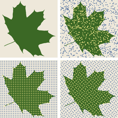
Illustration by Brian Hayes.
Tossing darts at random can be difficult and dangerous. But if you’re willing to accept dots in lieu of darts, and if you let the computer take care of sprinkling them at random, the leaf-measuring experiment is easy, and it works remarkably well.
I collected a leaf from a nearby sugar maple, photographed it, and placed the green shape within a square field of 1,024×1,024 blank pixels. Then I wrote a program that tosses random dots (actually pseudorandom dots) at the digitized image. The first time I ran the program, 429 of 1,024 dots fell on the leaf, for an area estimate of 0.4189. The actual area, as defined by a count of colored pixels, is 0.4185. The random-dots approximation was somewhat better than I expected—a case of random good luck, though nothing out of the ordinary. When I repeated the experiment 1,000 times, the mean estimate of the leaf’s area was 0.4183, with a standard deviation of 0.0153.
The basic idea in Monte Carlo studies is to reformulate a mathematical problem—such as calculating the area of a leaf—as a game of chance, where a player’s expected winnings are the answer to the problem. In simple games, one can calculate the exact probability of every outcome, and so the expected winnings can also be determined exactly. Where such calculations are infeasible, the alternative is to go ahead and play the game, and see how it comes out. This is the strategy of a Monte Carlo simulation. The computer plays the game many times, and takes the average result as an estimate of the true expected value.
For the leaf-in-a-square problem, the expected value is the ratio of the leaf area to that of the square. Choosing N random points and counting the number of “hits” approximates the area ratio, and the approximation gets better as N increases. When N approaches infinity, the measurement becomes exact. This last point is not just an empirical observation but a promise made by a mathematical theorem, namely the law of large numbers. This is the same principle that guarantees a fair coin will come up heads half the time when the sample is large enough.
Randomness has a conspicuous role in this description of the Monte Carlo method. In particular, the appeal to the law of large numbers requires that the sample points be chosen randomly. And it’s easy to see—just by looking at a picture—why random sampling works well: It scatters points everywhere. What’s not so easy to see is why other kinds of sample-point arrangements would not also serve the purpose. After all, one could measure the leaf area by laying down a simple grid of points in the square and counting the hits. I tried this experiment with my leaf image, placing 1,024 points in a 32×32 grid. I got an area estimate of 0.4209—not quite as good as my lucky random run, but still within 0.6 percent of the true area.
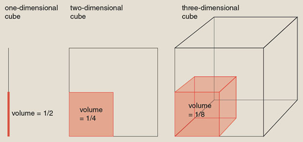
Illustration by Brian Hayes.
I also tried measuring the leaf with 1,024 quasirandom sample points, whose arrangement is in some sense intermediate between total chaos and total order. (For an explanation of how the quasirandom pattern is constructed, click the image below to see “A Recipe for Quasirandom Numbers.”) The estimate from counting hits with quasirandom points was 0.4141, giving an error of 1 percent.
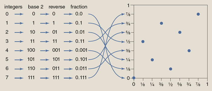
Illustration by Brian Hayes.
All three of these procedures give quite respectable results. Does that mean they are all equally powerful? No, I think it means that measuring the area of a leaf in two dimensions is an easy problem.
The task gets much harder in higher dimensions. Understanding why calls for an exercise in multidimensional thinking. Imagine a d-dimensional “cube” with edges of length 1, and a smaller cube inside it, with edge lengths along each dimension equal to 1/2. When d=1, a cube is just a line segment, and volume is equivalent to length; thus the smaller cube has half the volume of the large one. For d=2, the cube is a square, and volume is area; the small cube has volume 1/4. The case d=3 corresponds to an ordinary cube, and the volume filled by the small cube is now just 1/8. The progression continues. By the time we reach dimension d=20, the smaller cube—still with edge length 1/2 along each dimension—occupies only a millionth of the total volume. The mathematician Richard Bellman called this phenomenon “the curse of dimensionality.”
If we want to measure the volume of the one-in-a-million small cube—or even just detect its presence—we need enough sampling points to get at least one sample from the small cube’s interior. In other words, when we’re counting hits, we need to count at least one. For a 20-dimensional grid pattern, that means we need a million points (or, more precisely, 220=1,048,576). With random sampling, the size requirement is probabilistic and hence a little fuzzy, but the number of points needed if we want to have an expectation of a single hit is again 220. The analysis for quasirandom sampling comes out the same. Indeed, if you are groping blindly for an object of volume 1/2d, it hardly matters how the search pattern is arranged; you will have to look in 2d places.
If real-world problems were as hard as this one, the situation would be bleak. There would be no hope at all of dealing with a 360-dimension integral. But we know some problems of that scale do yield to Monte Carlo techniques; a reasonable guess is that the solvable problems have some internal structure that speeds the search. Furthermore, the choice of sampling pattern does seem to make a difference, so there is a meaningful distinction to be made among all the gradations of true, pseudo, quasi and non randomness.
The concept of randomness in a set of numbers has at least three components. First, randomly chosen numbers are unpredictable: There is no fixed rule governing their selection. Second, the numbers are independent, or uncorrelated: Knowing one number will not help you guess another. Finally, random numbers are unbiased, or uniformly distributed: No matter how you slice up the space of possible values, each region can expect to get its fair share.
These concepts provide a useful key for distinguishing between truly random, pseudorandom, quasirandom and orderly sets. True random numbers have all three characteristics: They are unpredictable, uncorrelated and unbiased. Pseudorandom numbers abandon unpredictability; they are generated by a definite arithmetic rule, and if you know the rule, you can reproduce the entire sequence. But pseudorandom numbers are still uncorrelated and unbiased (at least to a good approximation).
Quasirandom numbers are both predictable and highly correlated. There’s a definite rule for generating them, and the patterns they form, although not as rigid as a crystal lattice, nonetheless have a lot of regularity. The one element of randomness that quasirandom numbers preserve is the uniform or equitable distribution. They are spread out as fairly and evenly as possible.
A highly ordered set, such as a cubic lattice, preserves none of the properties of randomness. It’s obvious that these points fail the tests of unpredictability and independence, but perhaps it’s not so clear that they lack uniform distribution. After all, it’s possible to carve up an N-point lattice into N small cubes that each contain exactly one point. But that’s not enough to qualify the lattice as fairly and evenly distributed. The ideal of equal distribution demands an arrangement of N points that yields one point per region when the space is divided into any set of N identical regions. The rectilinear lattice fails this test when the regions are slices parallel to the axes.
These three aspects of randomness are important in different contexts. In the case of the other Monte Carlo—the casino in Monaco—unpredictability is everything. Cryptographic applications of randomness are similar. In both these cases, an adversary is actively trying to detect and exploit any hint of pattern.
Some kinds of computer simulations are very sensitive to correlations between successive random numbers, so independence is important. For the volume estimations under discussion here, however, uniformity of distribution is what matters most. And the quasirandom numbers, by giving up all pretense to unpredictability or lack of correlation, are able to achieve higher uniformity.
Uniformity of distribution is measured in terms of its opposite, which is called discrepancy. For points in a two-dimensional square, discrepancy is calculated as follows. Consider all the rectangles with sides parallel to the coordinate axes that could possibly be drawn inside the square. For each such rectangle, count the number of points enclosed, and also calculate the number of points that would be enclosed, based on the area of the rectangle, if the distribution were perfectly uniform. The maximum difference between these numbers, taken over all possible rectangles, is a measure of the discrepancy.
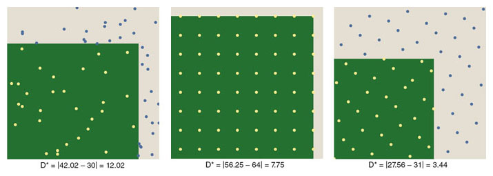
Illustration by Brian Hayes.
Another measure of discrepancy, called star discrepancy, looks only at the subset of axis-parallel rectangles that have one corner anchored at the origin of the unit square. And there’s no reason to consider only rectangles; versions of discrepancy can be defined for circles or triangles or other figures. The measures are not all equivalent; results vary depending on the shape. It’s interesting to note that the process for measurement of discrepancy has a strong resemblance to the Monte Carlo process itself.
Grids and lattices fare poorly when it comes to discrepancy because the points are arranged in long rows and columns. An infinitely skinny rectangle that should enclose no points at all can take in an entire row. From such worst-case rectangles it follows that the discrepancy of a square lattice with N points is √N. Interestingly, it turns out that the discrepancy of a random or pseudorandom lattice is also about √N. In other words, in an array of a million random points, there is likely to be at least one rectangle that has either 1,000 points too many or 1,000 too few.
Quasirandom patterns are deliberately designed to thwart all opportunities for drawing such high-discrepancy rectangles. For quasirandom points, the discrepancy can be as low as the logarithm of N, which is much smaller than √N. For example, at N=106, √N=1,000 but log N=20. (I am taking logarithms to the base 2.)
Discrepancy is a key factor in gauging the performance of Monte Carlo and quasi–Monte Carlo simulations. It determines the level of error or statistical imprecision to be expected for a given sample size. For conventional Monte Carlo, with random sampling, the expected error diminishes as 1/√N. For quasi–Monte Carlo, the corresponding “convergence rate” is (log N)d/N, where d is the dimensionality of the space. (Various constants and other details are neglected here, so the comparison is valid only for rates of growth, not for exact values.)
The 1/√N convergence rate for random sampling can be painfully slow. Getting one more decimal place of precision requires increasing N by a factor of 100, which means that a one-hour computation suddenly takes four days. The reason for this sluggishness is the clumpiness of the random distribution. Two points that happen to lie close together waste computer effort, because the same region is sampled twice; conversely, voids between points leave some areas unsampled and thereby contribute to the error budget.
Compensating for this drawback, random sampling has one very important advantage: The convergence rate does not depend on the dimension of the space. To a first approximation, the program runs as fast in 100 dimensions as in two dimensions. Quasi–Monte Carlo is different in this respect. If only we could ignore the factor of (log N)d, the performance would be dramatically superior to random sampling. We would have a 1/N convergence rate, which calls for just a tenfold increase in effort for each additional decimal place of precision. However, we can’t ignore the (log N)d part. This factor grows exponentially with increasing dimension d. The effect is small in dimension 1 or 2, but eventually it becomes enormous. In 10 dimensions, for example, (log N)10/N remains larger than 1/√N until N exceeds 1043.
It was this known slow convergence in high dimensions that led to surprise over the success of the Paskov and Traub financial calculation with d=360. The only plausible explanation is that the “effective dimension” of the problem is actually much lower than 360. In other words, the volume being measured doesn’t really extend through all the dimensions of the space. (In the same way, a sheet of paper lives in a three-dimensional space, but not much is lost by pretending it has no thickness.)
This explanation may sound dismissive: The calculation succeeded not because the tool was more powerful but because the problem was easier than it looked. But note that the effective reduction in dimension works even when we don’t know which of the 360 dimensions can safely be ignored. That’s almost magical.
How commonplace is this phenomenon? Is it just a fluke, or confined to a narrow class of problems? The answer is not yet entirely clear, but a notion called “concentration of measure” offers a reason for optimism. It suggests that the high-dimension world is mostly a rather smooth and flat place, analogous to a high-gravity planet where it costs too much to create jagged alpine landscapes.
The Monte Carlo method is not a new idea, and neither is the quasi–Monte Carlo variation. Simulations based on random sampling were attempted more than a century ago by Francis Galton, Lord Kelvin and others. In those days they worked with true random numbers (and had a fine time generating them!).
The Monte Carlo method per se was invented and given its name at the Los Alamos Laboratory in the years after World War II. It’s no surprise that the idea emerged there: They had big problems (even more frightening than collateralized mortgage obligations); they had access to early digital computers (ENIAC, MANIAC); and they had a community of creative problem-solvers (Stanislaw Ulam, John von Neumann, Nicholas Metropolis, Marshall Rosenbluth). From the outset, the Los Alamos group relied on pseudorandom numbers. At the first conference on Monte Carlo methods, in 1949, von Neumann delivered his famous quip: “Anyone who considers arithmetic methods of producing random digits is, of course, in a state of sin.” Then he proceeded to sin.
Quasi–Monte Carlo was not far behind. The first publication on the subject was a 1951 report by Robert D. Richtmyer, who was head of the theoretical division at Los Alamos. The paper is an impressive debut. It sets forth the motivation for quasirandom sampling, introduces much of the terminology, and explains the mathematics. But it was also presented as an account of a failed experiment; Richtmyer had wanted to show improved convergence time for quasi–Monte Carlo computations, but his results were negative. I am a fervent believer in reporting negative results, but I have to concede that it may have inhibited further investigation.
In 1968 S. K. Zaremba, then at the University of Wisconsin in Madison, wrote a strident defense of quasirandom sampling (and a diatribe against pseudorandom numbers). As far as I can tell, he won few converts.
Work on the underlying mathematics of low-discrepancy sequences has gone on steadily through the decades (most notably, perhaps, by Klaus Friedrich Roth, I. M. Sobol, Harald Niederreiter and Ian H. Sloan). Now there is renewed interest in applications, and not just among the Wall Street quants. It’s catching on in physics and other sciences as well. Ray-tracing in computer graphics is another promising area.
The shifting fortunes of pseudo- and quasirandomness might be viewed in the context of larger trends. In the 19th century, randomness of any kind was an unwelcome intruder, reluctantly tolerated only where necessary (thermodynamics, Darwinian evolution). The 20th century, in contrast, fell madly in love with all things random. Monte Carlo models were a part of this movement; the quantum theory was a bigger part, with its insistence on divine dice games. Paul Erdös introduced random choice into the methodology of mathematical proof, which is perhaps the unlikeliest place to look for it. In computing, randomized algorithms became a major topic of research. The concept leaked into the arts, too, with aleatoric music and the spatter paintings of Jackson Pollack. Then there was chaos theory. A 1967 essay by Alfred Bork called randomness “a cardinal feature of our century.”
By now, though, the pendulum may be swinging the other way, most of all in computer science. Randomized algorithms are still of great practical importance, but the intellectual excitement is on the side of derandomization, showing that the same task can be done by a deterministic program. An open question is whether every algorithm can be derandomized. Deep thinkers believe the answer will turn out to be yes. If they’re right, randomness confers no essential advantage in computing, although it may still be a convenience.
Quasirandomness seems to be taking us in the same direction, with a preference for taking our drams of randomness in the smallest possible doses. What’s ahead may be a kind of homeopathic doctrine, where the greater the dilution of the active agent, the greater its potency. That’s nonsense in medicine, but perhaps it works in mathematics and computation.
©Brian Hayes
Click "American Scientist" to access home page
American Scientist Comments and Discussion
To discuss our articles or comment on them, please share them and tag American Scientist on social media platforms. Here are links to our profiles on Twitter, Facebook, and LinkedIn.
If we re-share your post, we will moderate comments/discussion following our comments policy.