Rapid Climate Change
By Kendrick Taylor
New evidence shows that earth's climate can change dramatically in only a decade. Could greenhouse gases flip that switch?
New evidence shows that earth's climate can change dramatically in only a decade. Could greenhouse gases flip that switch?

DOI: 10.1511/1999.30.320
Over the course of geologic history, the earth's environment has been far from static. Indeed, 600 million years ago the atmosphere lacked sufficient oxygen to support animal life. More recently, as shown by sediments recording conditions over the past 500,000 years, the planet's climate varied between at least two different states.
The record from the past 150,000 years is particularly well preserved, offering details about these repeated climate changes. Between about 131,000 and 114,000 years ago there was a warm period like today's climate, referred to in Europe as the Eemian or globally as Marine Isotope Stage 5e. This was followed by the Wisconsin ice age, which ended about 12,000 years ago when the current relatively warm Holocene period began.
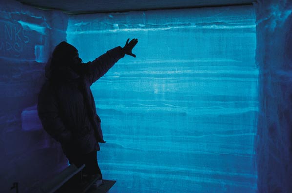
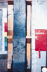
Photograph by Kendrick Taylor
Although the past half-million years constitutes the current-events period in geologic time, on a human time scale the events I just described are in the distant past. Because their time scales are so long, I used to believe that changes in climate happened slowly and would never affect me. After all, a single climate cycle that includes an ice age and a warm period lasts 150,000 years and is controlled by gradually changing orbital parameters of the earth. It did not seem possible that climate cycles that lasted so long could change perceptibly during my lifetime. Even greenhouse-induced climate changes are normally predicted to happen gradually over several generations, allowing an opportunity for society to adapt.
My attitude changed profoundly while I was working on a project funded by the National Science Foundation to develop a climate record for the past 110,000 years. By examining ice cores from Greenland, my colleagues and I determined that climate changes large enough to have extensive impacts on our society have occurred in less than 10 years. Now I know that our climate could change significantly in my lifetime. We are still a long way from being able to predict such a change, but we are getting closer to understanding how it might take place. A pressing concern is whether anthropogenic changes to our planet's atmosphere might perturb the climate's stability.
One can learn a lot about what controls climate by studying glacial ice. When snow falls, it collects insoluble dust particles, soluble compounds and the water in the snow itself. In some places more snow falls in a year than melts or sublimates away. Annual layers of snow pile up, with atmospheric gases filling the open pores between snow crystals. The weight of accumulating snow compresses the pores in the snow below, turning the snow into ice and trapping the atmospheric gases. The dust, chemicals and gases in the ice reflect the environment along the water's journey from distant sources to the glacier. They record how cold it was, how much snow fell in a year, what the concentration of atmospheric gases was and what the atmospheric circulation patterns were.
We can identify annual layers in the ice because the concentration of sea salts, nitrate and mineral dust and the gas content in winter snow are different than in summer snow. We count the annual layers to determine the age of the ice, and by measuring the thickness of the annual layers we can determine how much snow fell each year. The gas trapped between ice crystals offers a sample of the ancient atmosphere, and we can use it to determine what the concentrations of greenhouse gases such as carbon dioxide and methane were long before human beings measured the atmosphere directly. General patterns of atmospheric circulation can be reconstructed by using tracers such as soluble chemicals (for example, nitrate, ammonium, sodium and calcium) and rare earth elements in insoluble dust particles to determine how wind moved air and dust from the source regions for these compounds to the drilling site.
Air temperature is naturally of primary interest when we talk about climate, and fortunately we have three ways to determine what it was in the past. First, we can measure the isotopic composition of the oxygen and hydrogen in the ice. When water vapor in clouds condenses, the ratio of oxygen-18 to oxygen-16 and the hydrogen-2/hydrogen-1 ratio are affected by the ambient temperature; the colder the cloud, the lower the ratio. Measuring how the ratios of these isotopes changes along an ice core gives us a good idea how the air temperature changed over time.
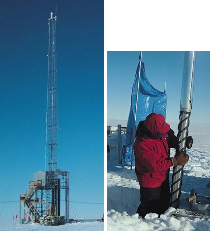
Photograph by Kendrick Taylor
The second way to determine prehistoric temperatures is to measure the isotopic composition of the nitrogen gas trapped in the ice. At depths between about 5 and 50 meters in an ice sheet, air can move in interconnected pores but is sheltered from mixing by the wind. Nitrogen-15 slowly moves toward colder locations, and nitrogen-14 slowly moves toward warmer locations. This process creates a near-surface gradient in the nitrogen-15/nitrogen-14 ratio that depends on the near-surface temperature gradient. The resulting isotopic composition of the nitrogen trapped in the ice depends on the difference between the surface temperature and the temperature at depth at the time when the ice overburden pressure closes the pores and traps the nitrogen gas in the ice. Variations in the isotopic composition of the nitrogen along a core show when and by how much the surface temperature changed.
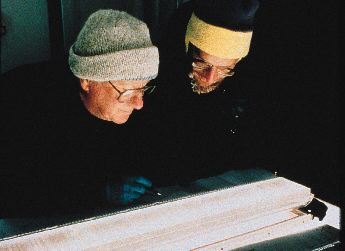
Photograph courtesy of Ken Abbott/National Ice Core Laboratory
Finally, because of the large thermal inertia of an ice sheet, the current temperature distribution in an ice sheet is strongly influenced by what the surface temperature was in the past. The physics is similar to cooking a large frozen turkey. If we move the turkey directly from the freezer into the oven, the outside of the turkey will be done before the inside even defrosts. By modeling the current thermal state of the turkey, or an ice sheet, we can determine the history of the turkey's, or ice sheet's, surface temperature. The physics of these three approaches is well understood; together they allow us to reconstruct how the surface temperature changed during the past several hundred thousand years.
In Greenland, annual ice layers are stacked up like thousands of annual weather reports. In 1982, a European and American team made the first attempt to read that record, by recovering an ice core from southern Greenland. Measurements on the ice core indicated that about 11,700 years ago the climate of the North Atlantic region changed from a dry and cold ice age to the current warmer and wetter Holocene. Altogether it took 1,500 years for the climate transition to be complete and a few thousand more years to melt most of the ice, but the surprise was that most of the transition occurred in only 40 years. This was only one record, and it came from a single 10-centimeter-diameter ice core. Still, this finding was impossible to ignore and too puzzling to comprehend.
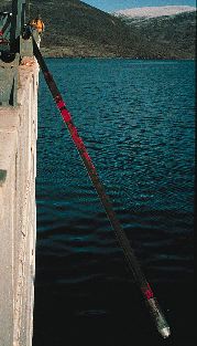
Photograph courtesy of Anne Jennings
In 1993, Americans and Europeans led by Paul Mayewski of the University of New Hampshire and Bernhard Stauffer of the University of Bern in Switzerland finished recovering two new ice cores from the summit of the Greenland ice sheet. More than 40 university and national laboratories participated in the projects. We shared samples, spent time in one another's labs, replicated one another's results, proposed ideas, tore them apart and then jointly proposed better ones.
Photograph courtesy of Bedford Institute of Oceanography
One of the justifications for these new cores, located 30 kilometers apart, was to verify and learn more about the 40-year change in climate, an event observed in both cores. The records stored in these cores were more detailed than before and showed that within a 20-year period at the summit of Greenland, where ice is thickest, the amount of snow deposited each year doubled, average annual surface temperature increased by 5 to 10 degrees Celsius and wind speeds increased. The same ice cores also showed that the spatial extent of sea ice decreased, atmospheric-circulation patterns changed, and the size of the world's wetlands increased. Many of these shifts in parameters, including at least a 4-degree Celsius increase in the average annual air temperature, happened in less than 10 years. These changes were not restricted to Greenland; the global nature of many of these ice-core records showed that low-latitude, continental-scale regions rapidly got warmer and wetter. The most dramatic change occurred 11,700 years ago. But we also found comparable anomalies every several thousand years during the Wisconsin ice age (see Figure 6). Further, Antarctic ice cores also show comparable climate transitions at these times.
One can also learn a lot about what controls climate by studying sediments on the ocean floor. These sediments contain the decayed remains of ocean organisms and inorganic material from the erosion of rocks. Ocean organisms assimilate chemical compounds from the water as they grow, and the compounds they incorporate are partially determined by the environment in which they live. Thus the decayed remains of the organisms that fall to the ocean floor contain a record of what chemical compounds were available and the temperature of the water in which they lived.
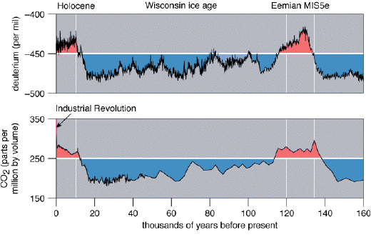
Drawing by Edward Roberts. Deuterium data from J. Jouzel, Laboratoire de Modélisation du Climat et de l’Environnement, France. CO2 data, from direct observations and three different ice cores, come from C. Keeling, Scripp’s Institution of Oceanography; A. Indermuhle and A. Neftal, University of Bern; and J. Barnola et al., Laboratoire de Glaciologie et Géophysique de l’ Environnement, France
For example, consider an ocean-sediment core collected at Bermuda Rise, a place where ocean currents deposit a lot of sediment. The oxygen-18/oxygen-16 ratio of seawater varies through time depending on how much water is locked in ice sheets and how much water is in the ocean (see Figure 7). The near surface–dwelling foraminiferan Globigerinoides ruber uses seawater to make its shell. By measuring the oxygen isotopic composition of the shells recovered from an ocean core, we can determine how much water was locked up in ice sheets when the foraminiferan was living. Likewise, the bottom-dwelling foraminiferan Nutallides umbonifera incorporates cadmium and calcium in its shell. By measuring the ratio of cadmium to calcium in the shells recovered from an ocean core, we can tell where the bottom water came from when the foraminiferan was living. High values of the cadmium-to-calcium ratio indicate that the water near the bottom came to the Bermuda Rise from the south, whereas a low ratio indicates that the bottom water came from the north.
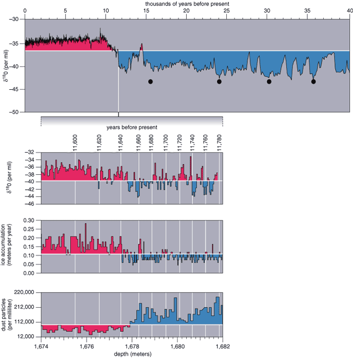
Drawing by Edward Roberts. Age data from D. Meese, CRREL; oxygen-18 data from J. White, University of Colorado; ice accumulation data from R. Alley, Pennsylvania State University; dust concentration data from G. Zielinski, University of New Hampshire
Ocean sediments also contain ground-up rock, which is transported and deposited by ocean currents, just as wind carries airborne dust to be deposited on ice sheets. The mineralogy of the ground-up rock can be used to identify where it came from. For example, a layer of hematite-rich sediments in ocean cores near Bermuda indicates that ocean currents were transporting material from the east coast of Canada to Bermuda when the sediments in the layer were deposited.
To determine what the temperature of the ocean surface was in the past we can use organic compounds made by phytoplankton. Phytoplankton live near the ocean surface where there is light for photosynthesis. Some phytoplankton produce compounds know as alkenones, which are straight chains of carbon atoms. Along these chains of carbon there can be two or three double bonds. The number of double bonds depends on the water temperature. The double bonds are thought to keep the cell membrane pliable in cold water. When the phytoplankton die, the alkenones fall to the bottom and become incorporated into the sediment. By measuring the ratio of different types of alkenones we can determine what the surface water temperature was when the phytoplankton were living.
By collecting cores of the ocean sediments at different locations, we can determine a lot about how the ocean circulated water and heat in the past. The rapid climate changes recorded in the ice cores encouraged a search for ocean sediment records with high time resolution. In the past few years locations have been identified in the ocean where sediment accumulates rapidly, and the sediment cores from these locations have comparable time resolution to the ice cores. Coring projects off the coast of Bermuda by Konrad Hughen, Julian Sachs and Scott Lehman with the University of Colorado, in conjunction with Lloyd Keigwin of Woods Hole Oceanographic Institution and Ed Boyle of the Massachusetts Institute of Technology, found the same rapid changes in climate as were recorded in the ice cores. Other groups have found similar records near Santa Barbara, California and off the coast of India.
Paleoclimatic evidence worldwide shows that a global change in climate took place 11,700 years ago, and in the North Atlantic a large part of the change took less than 20 years. It was a few thousand years before the completion of the transition from ice age to warm period; still, in just a 20-year period the climate of a large part of the earth changed significantly. There was no warning. A threshold was crossed, and the climate in much of the world shifted abruptly from cold to warm. This was not a small perturbation; our civilization has never experienced a climate change of this magnitude or speed. To get an idea of what happened, imagine that over a 20-year period the weather at your home became that typical of a place 400 to 600 miles farther south. What might be the mechanism for so rapid and large a climate change?
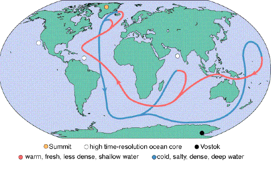
Like the atmosphere, the oceans are far from static. Currents, of which the Caribbean-Atlantic Gulf Stream is just a small part, continually exchange water among all the oceans and between the surface and the depths. For the sake of convenience, we shall start this journey in the Gulf Stream, where water moves northward along the East Coast of the U.S. toward Iceland. Along the way, the water exchanges heat with the air, warming the air and cooling the water in the process. Water evaporates from the surface and leaves behind dissolved salt. The combination of chilling and evaporation makes surface water denser as it moves north. In the vicinity of Iceland, the surface water becomes denser than the water below it and sinks. This dense, cold water then moves south along the bottom of the Atlantic, around the Horn of Africa and, still near the bottom, continues to the North Pacific, where it upwells to the surface. Surface water in the North Pacific makes room for the upwelling bottom water by moving south, passing between Asia and Australia and finally catching the tail of the circulation pattern at the beginning of the Gulf Stream in the Atlantic off Central America (see Figure 8). For most of its journey, the surface water collects heat and freshwater, which makes the surface water more buoyant than the water underneath it. But in the North Atlantic, the combination of cold temperatures and evaporation makes the water dense again and it sinks.
Wally Broecker of Columbia University likens this circulation pattern to a long conveyor belt that moves water, salt and heat. He was among the first to recognize that alterations in the path of the ocean conveyor belt would change climate in much the same way that turning off the furnace fan changes the temperature distribution in a house. He proposed that the large oscillations in climate observed in the geologic record were caused by different patterns of ocean circulation.
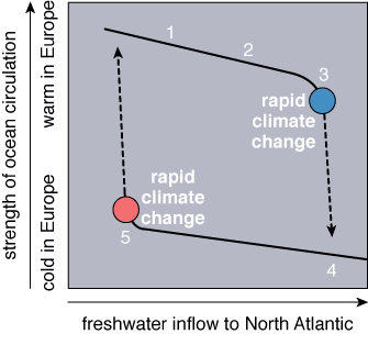
Because the oceans must abide by the constraints of geography and the laws of physics, there are only a few patterns in which the oceans can circulate. At a recent conference organized by Robert Webb of NOAA and Peter Clark of Oregon State University, climate scientists identified three modes of ocean circulation, each of which is associated with a different climate. The current mode produces the warmest conditions in the North Atlantic. Surface water sinks in two regions of the North Atlantic, and a large volume of surface water and heat is drawn from the tropics to replace the sinking North Atlantic water. The heat carried north by the northward-moving surface water warms eastern North America, the North Atlantic and most of Europe. The second mode of ocean circulation occurs when surface water sinks in only one area of the North Atlantic. Less surface water sinks to the bottom, so smaller amounts of warm surface water and heat are drawn north to replace the sinking water. This mode was in place during the warmest times of the Wisconsin ice age, when climate was only slightly colder than current conditions. In the coldest mode, no water sinks in the North Atlantic; hence no warm water is drawn north. This was the condition during the coldest portions of the Wisconsin ice age.
Each of these modes of ocean circulation is associated with a small range of prevailing environmental conditions. Weather anomalies such as 10-year-long droughts or wet periods, as significant as they may seem to human affairs, are a reflection of the small range of environmental conditions associated with a single mode of ocean circulation. If, however, environmental conditions are externally forced to be inconsistent with the existing mode of ocean circulation, the circulation will switch to a mode that is more consistent with those environmental conditions. An example of this forcing would be a change in the amount of solar heat reaching, and retained at, the earth's surface. Such a change could be the result of alterations either in solar output or in the way the atmosphere regulates the exchange of heat between the earth's surface and space. The transitions between different modes of ocean circulation are abrupt. The ocean-sediment cores and ice cores tell us that they frequently take only several decades or less.
Numerical models of ocean circulation developed by Thomas Stocker of the University of Bern and Syukuro Manabe of Princeton University show that each circulation mode is stable for a particular range of environmental conditions. For example, if the discharge of a river changes, altering the density of the surface water in the adjoining ocean, the ocean-circulation pattern will change only if it is unstable under this new set of conditions. As long as the climate system stays within the stable-mode range, river discharge and greenhouse-gas concentration can vary without having much influence on climate.
Drawing by Edward Roberts
Stefan Rahmstorf of the Potsdam Institute for Climate Impact Research has used numerical models to show how surprisingly sensitive ocean circulation can be to changes in freshwater discharge. His numerical models show that if the climate system is near the threshold between stable modes, a small change in the amount of freshwater entering the North Atlantic will force a large and rapid shift to a different ocean-circulation pattern. Like a coin on edge, which topples with only a breath of air, an unstable pattern quickly assumes a new position where it becomes quite stable. The climate changes recorded by the ice and ocean-sediment cores appear to have taken place when some crucial threshold was crossed, resulting in large and rapid switches—in geologic time, like the flip of a switch—in ocean circulation.
Unfortunately, no one knows yet what caused this switch to flip. We know of external forcing mechanisms, but their time periods do not match the record. For example, the distribution of solar energy reaching the earth varies according to the relative positions of the sun and earth. These variations, called Milankovitch cycles, have periods of tens of thousands of years and are thus too slow to explain the rapid changes seen every couple of thousand years during the Wisconsin ice age. The Milankovitch cycles define the big picture and determine when changes could occur, but some smaller, quicker-acting mechanism triggered the more frequent switches during the Wisconsin.
The leading idea, which has been simulated in computer models, is that increased discharges of freshwater glacial ice and river runoff into the North Atlantic reduced the density of the surface water enough that it could not sink. This slowed the ocean conveyor, forcing it to switch to another circulation pattern. Other emerging concepts place the source of the disruption of the conveyor in the tropical Pacific. Variability in the sun's output is another possible cause of the climate variations, but the record of solar output is not good enough to adequately investigate this idea. Furthermore, the dynamics of ocean circulation around Antarctica are too poorly understood to completely exclude the possibility that they may play a role. Whatever the cause may be, it is worrisome that the phenomenon that has repeatedly triggered major changes in ocean circulation and the earth's climate is so subtle that we have not been able to identify it. This emphasizes how large changes in the interaction of the oceans, atmosphere and ice sheets have been triggered by small perturbations of the environment.
Human beings have made major modifications to the earth's environment in little more than a century, increasing the concentration of carbon dioxide in the atmosphere to its highest level in 260,000 years. Numerical models can be used to estimate what will happen when anthropogenic increases in the atmospheric concentration of gases such as carbon dioxide and methane block heat from leaving the earth. The increased concentration of these gases acts like a greenhouse, and the average temperature of the earth gets warmer. But the numerical models of Stocker, Rahmstorf and others suggest there may be surprises in the greenhouse.
When the greenhouse effect warms the earth, it accelerates the hydrologic cycle, more water moves around in the atmosphere, and rainfall increases in many places. Some models suggest that this will slowly decrease the salinity of the North Atlantic, making the surface water less dense. Were a critical density threshold to be crossed, ocean circulation would abruptly switch to a new stable mode.
This would be more than just a switch in ocean circulation; it would be a switch in the way tropical heat is transported to the North Atlantic. At the least, Northern Europe and Scandinavia would be 2 to 5 degrees colder on average than they are now, and the amount of precipitation would decrease dramatically. It would not necessarily be a rapid return to an ice age, but it might be a start in that direction. The orbital parameters of the earth are such that we are due for another ice age, and a cooling in the north Atlantic at a time when orbital parameters favor a return to a much colder climate could be the trigger that initiates such a change.
Drawing by Edward Roberts. Adapted from work by Stefan Rahmstorf, Potsdam Institute for Climate Impact Research, Germany
A switch in climate from a warm period (like the current Holocene epoch) to an ice age has happened before. Ocean and lake cores tell us that the warm Eemian period from about 131,000 to 114,000 years ago—when the distribution of ice sheets was similar to what it is today—switched to the Wisconsin ice age in no more than 400 years, the minimum time resolution of the record from these ancient sediments. Unfortunately, we have yet to recover an ice core that shows in sharp detail how the Eemian Period ended. This is old ice. It is difficult to find a place where it snowed enough to produce a high time-resolution record but not so much as to smear the record against the bedrock. An international project, led by Claus Hammer of the University of Copenhagen, has identified the most likely location in Greenland for this ice to be found and is collecting a core.
Many arctic ice cores tell us that 8,200 years ago the climate approached ice age conditions for a 400-year period before returning to conditions similar to today. This excursion was most likely caused by the one-time draining of lakes left behind by the melting of the Canadian ice sheets. This change in freshwater flux to the oceans was large but not that much different from what greenhouse-induced changes may produce in the future. The fact that it took place when climate conditions were similar to today demonstrates that large and rapid climate switches do not happen exclusively when there are extensive northern hemisphere ice sheets. It is ironic that greenhouse warming may lead to rapid cooling in eastern North America, Europe and Scandinavia, and it is possible that altered ocean circulation could lead to much larger changes. We have no experience predicting climate switches between stable modes, so it would be wise to expect surprises.
Climate is the result of the exchange of heat and mass between the land, ocean, atmosphere, ice sheets and space. As long as changes to the land, ocean, atmosphere and ice sheets stay below the thresholds I have just described, climate changes will happen slowly. But the climate will change rapidly if those thresholds are crossed. So rapidly that it would be impossible to rearrange agricultural practices quickly enough to avoid stressing world food supplies. So rapidly that many species would not be able to adapt, because their habitat, already greatly reduced by human activities, would be eradicated.
Human ingenuity would most likely allow us to adapt to a rapid change in climate, but we would pay a larger price than our civilization has ever known. Imagine the economic and social cost of moving, in a 20-year period, most of our agricultural activities 500 miles south of their current locations. Imagine the social cost and famine if agriculture could not be relocated quickly enough. Even a short-duration event such as the Dust Bowl years in the 1930s had a large influence on American society. The Little Ice Age, which caused major resettlement in Europe in the 15th and 16th centuries, is a more likely analogue of where we might be headed.
Some have proposed that we could counterbalance the greenhouse effect by manipulating the global exchanges of heat and mass. Methods that have been discussed include blocking the Strait of Gibraltar to change the salinity of the North Atlantic, using airplane-distributed particles or large orbiting sunshades to shade the earth, and fertilizing the ocean with iron to promote production of carbon dioxide-consuming biomass. But we have a poor record of managing even small ecosystems and lack a complete understanding of the ocean-atmosphere interactions that govern our climate. Intentionally manipulating climate would not only be costly and imprecise; it would also be impossible to benefit some regions without adversely effecting others. It would be a risky experiment on the only planet we can call home.
Although we do not know the critical level of greenhouse-gas concentration, we do know that reducing the rate of greenhouse emissions would help in two ways. First, the atmospheric concentration of greenhouse gases would increase more slowly. Second, numerical models by Thomas Stocker and Andreas Schmittner of the University of Bern and others predict that the climate threshold will occur at a higher concentration of greenhouse gases if the concentration of greenhouse gases increases slowly. Slowing the rate of greenhouse-gas emissions would buy us more time to understand the consequences of our actions and might allow us to increase greenhouse-gas concentrations to a higher level before reaching the critical threshold.
It is true that computer models are not perfect; they indicate general patterns. And we need to improve our understanding in many areas before the models can pinpoint thresholds. For example, our understanding of the details of ocean circulation is poor, and the physics of cloud formation and their influence on heat exchange is elusive. When we model previous switches in climate, we can compare the model to the results of real-world experiments recorded in ocean sediments and ice cores. But when we model the future, we have no empirical basis to judge the model's accuracy. If we take no action until we are completely confident the models are correct, then the only use for the models will be to explain what happened. Our insistence on a tested model is part of the reason society is continuing to conduct the largest experiment ever done, the experiment of increasing the atmospheric concentration of greenhouse gases.
It will be another 20 years before the climate changes that are predicted to be associated with the greenhouse effect become large enough to be unambiguously differentiated from naturally occurring variations in climate. As a society we have the choice of ignoring the warning signs that our studies have uncovered or taking some action.
I think we should spend the next 20 years aggressively investigating our options. We should continue to focus on improving our ability to predict climate change. At the same time, we should test the technologies and polices we might need to reduce greenhouse-gas emissions, implementing them on a small scale where there would be minimal economic and social disruption. I am not alone among scientists in anticipating that 20 years from now our society may have to choose between disruptions associated with our current approach to energy use and disruptions associated with adopting an approach to energy use that produces fewer greenhouse gases. Procrastination will prevent making an informed decision and will increase the social and economic costs.
Click "American Scientist" to access home page
American Scientist Comments and Discussion
To discuss our articles or comment on them, please share them and tag American Scientist on social media platforms. Here are links to our profiles on Twitter, Facebook, and LinkedIn.
If we re-share your post, we will moderate comments/discussion following our comments policy.