Mud Acoustics
By Charles W. Holland, Stan E. Dosso, Jason D. Chaytor
Imaging the ocean requires an understanding of how different seafloor sediments interact with sound waves.
Imaging the ocean requires an understanding of how different seafloor sediments interact with sound waves.

Long before kindergarten, many of us experimented with mud. Its squishiness, the fact that we could launch airborne blobs with a kick or a stomp—and the satisfying thwuuck sounds that this activity made—provided hours of delightful exploration, sometimes despite protests from our parents. Although most kids outgrow playing in mud, some of us who study sound propagation in the ocean continue to be fascinated by it.
One might well ask, why is mud acoustics interesting and important? The answers are: We live on a muddy planet because oceans cover 70 percent of the Earth and mud covers the vast majority of the seabed; acoustics play a critical role in studying and operating in the oceans because light and radio waves are poorly transmitted in seawater, whereas sound propagates effectively; and acoustic waves in the ocean often interact with and are strongly affected by the seabed. Hence, measuring and understanding the acoustically relevant geophysical properties (or geoacoustic properties) of mud is necessary for applying and predicting acoustics in marine environments. But first, we need to define what is meant by the term mud.
Marine sediments can generally be divided into two broad categories: granular or coarse-grained sediments (such as sand or gravel) in which the individual grains are held together by gravitational forces, and fine-grained sediments (muds) in which the grains are held together primarily by electrochemical forces. More specifically, mud is an unconsolidated sediment that must have two components: some amount of microscopic material, be it clay-sized (less than 4 micrometers in diameter) or silt-sized (4 to 63 micrometers in diameter) grains, and water. Beyond these two requirements, mud may contain almost anything else of any size, such as sand and gravel, organic matter, and microplastics, often making it difficult to determine exactly what is meant when mud is used in scientific or engineering applications.
So perhaps it is easier to describe what mud is not, because other sediments are well-defined. Sediment that is either predominantly (nominally more than 50 percent by weight) composed of sand-sized (63 micrometers to 2 millimeters) or gravel-sized (more than 2 millimeters) material is not mud. Although sand- or gravel-dominated sediments may be described as “muddy” if they have clay- or silt-sized grains incorporated into them, they are not considered to be mud.
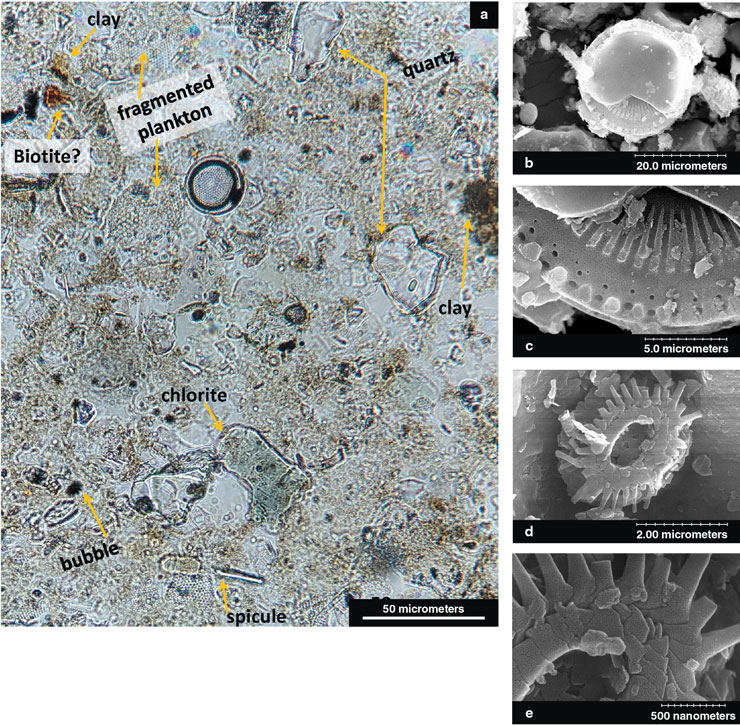
Acoustics Today 20:37–45 (a); adapted from J. T. Dubin et al., 2017 (b-e).
The figure above shows an optical image of mud. The larger greenish, brown, and clear grains are minerals worn away from preexisting rocks through weathering and erosion. There is also abundant biogenic silt (particles produced by living organisms) including diatoms, fragmented plankton shells (the fragments with many closely spaced holes), spicules (long needlelike features), clay, and possibly organic matter (shown as disseminated brown material).
The composition of the materials in a mud is vitally important to its geoacoustic properties. Beyond the requirement for water, the composition of mud is primarily a function of the environment in which it occurs. Muds in land-based and marine settings contain a mix of inorganic and organic components that can be derived from local or distant sources. Inorganic components are further divided into minerals from the weathering of nearby rocks, material that has been transported (such as volcanic ash), biogenic materials, and other minerals formed in place by chemical processes. These mineral and biogenic grains have a stunning range of shapes and sizes, from platy clays (which are formed by layers or sheets of crystals) to the exotic chambered and ornamented remains of microscopic marine organisms.
In general, inorganic components tend to dominate the composition of mud. This makeup is the case for a large area of biogenic ooze off the coast of Italy that almost entirely consists of the carbonate or silica fossil remains of single-celled marine algae (85 percent of which are clay-sized). A very different mud composed primarily of land-based grains (15 percent clay-sized) is found in an area known as the New England Mud Patch, located 95 kilometers south of Martha’s Vineyard, Massachusetts, and another site of extensive field studies.
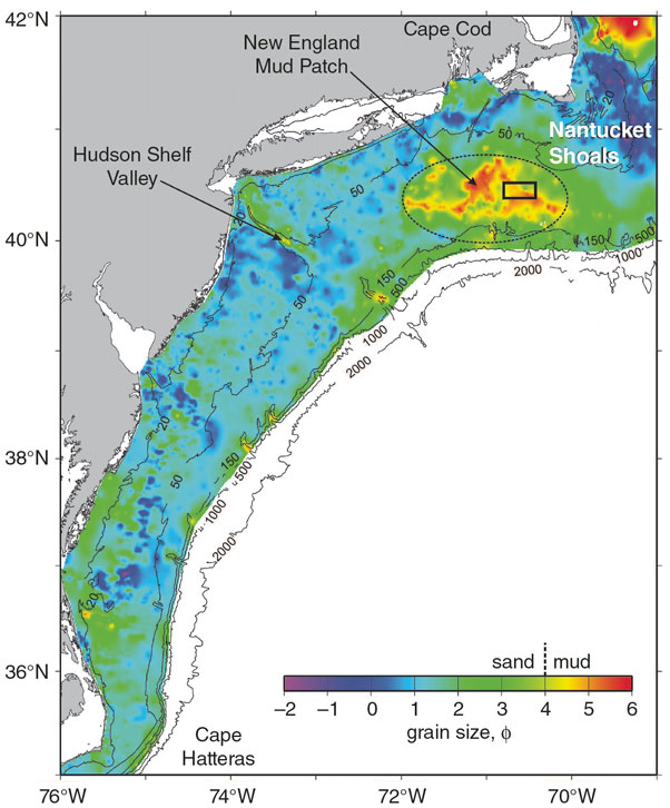
Adapted from J. A. Goff et al., 2019.
Organic components found in mud come from land-based plant and animal sources and marine organisms (such as bacteria, plankton, and larger mobile fauna) that undergo various levels of degradation. The decomposed organic matter may suspend silt and clay particles in the sediment fabric or, in other words, restrict the silt and clay particles from touching one another. The organic matter can also adsorb onto mineral surfaces and reside between mineral contact points. Gabriel Venegas of the University of New Hampshire and his colleagues have shown that all these interactions alter mud properties, decreasing stiffness, increasing viscosity, and decreasing density. In addition, Kelly M. Dorgan of the Dauphin Island Sea Lab in Alabama and her colleagues have demonstrated that biologic processes further alter mud geoacoustic properties through events such as burrowing and tube building by organisms that live on the seafloor.
The geoacoustic properties of marine sediments that are generally most important in influencing ocean-acoustic propagation are the speed of the sound waves, the loss of energy (or attenuation) of the sound waves, and the density of the sediments. When acoustic waves enter sediment, they create elastic movement that temporarily deforms the material, which produces what are called shear waves. The speed and attenuation of these shear waves in mud can be important in some cases; however, mud shear-wave speeds near the water–sediment interface are typically about two orders of magnitude smaller than the sound speed in mud or water, and, hence, there is little coupling between acoustic and shear waves. Thus, in many cases, it is a reasonable approximation from an acoustics perspective to model mud as what is called a lossy fluid, meaning that it loses some energy from the sound as the waves travel through it.

Adapted from J. A. Goff et al., 2019.
Sound speed and attenuation in muds and other sediments vary with the frequency of the acoustic waves passing through them. Measuring and understanding these frequency dependencies are challenging but important tasks because they provide clues about the underlying physics that control acoustic-wave propagation in sediments. Geoacoustic properties also depend on the depth below the water–sediment interface. This dependence is important because if the sound speed increases with depth, acoustic waves can be refracted or reflected upward back into the water column. Alternatively, if the sound speed decreases with or is independent of depth, the acoustic energy transmitted into the sediment does not return to the water column.
Geoacoustic properties of muds and other seabed sediments can be determined using two broad approaches: measured directly using invasive procedures (such as inserting a probe into the sediments or extracting a sediment sample, referred to as a core, for subsequent laboratory measurements), or inferred remotely using water-column measurements of acoustic fields that interact with the seabed. Direct and remote approaches are both important in developing our understanding of mud, and each has its own advantages and limitations.
For direct methods, sound speed and density are routinely measured in cores, whereas attenuation measurements are less common. Probes normally measure sound speed. Although useful information about mud is obtained with direct measurements, limitations on such methods include: the unavoidable disturbance and modification of sediment properties from their natural state, especially for muds that are often structurally fragile; restricted sampling depth, with most cores for acoustic purposes penetrating less than 10 meters and commonly about 1 meter, and probes penetrating up to about 3 meters; and the restricted range of high measurement frequencies, with probes operating in the range of single-digit kilohertz to hundreds of kilohertz and core measurements at hundreds of kilohertz. Despite these limitations, an important advantage of coring is that it retrieves the sample, which then can be studied minutely, including for underlying physical properties such as the mineralogy, chemistry, grain-size distribution, and organic matter content. These observations can be crucial for developing a fundamental understanding of the relationships between the physical and the geoacoustic properties of sediments.
In contrast to direct methods, remote-sensing methods infer sediment geoacoustic properties from measurements of acoustic fields that have been altered by interactions with the seabed and, hence, carry information on seabed properties. Remote-sensing methods require a theoretical model for these interactions such that acoustic data can be computed and predicted when given a set of geoacoustic properties, with the goal of determining property values for which the predicted data match the measured data. This remote-sensing procedure is referred to as geoacoustic inversion.
A variety of at-sea survey methods can be used to obtain different types of acoustic data that can be employed in geoacoustic inversions. The procedure can be based on measurements of either long-range or short-range acoustic propagation. Long-range methods, in which the propagation path is typically 1 to 10 kilometers long on the continental shelves, involve multiple or continuous acoustic bottom interactions and provide geoacoustic estimates that represent a lateral average of the sediment properties over the propagation path. Such methods are well-suited for estimating sediment properties for regional models and for long-range propagation predictions. A limitation, however, is that unknown spatial and temporal fluctuations in the environment of the water column or the seabed along the path can lead to biases in the inferred properties. Furthermore, detailed sediment-column structure may not be resolved because of this averaging, and intrinsic attenuation can be obscured by other cumulative loss mechanisms such as scattering from rough interfaces or volume heterogeneities. Thus, the detailed structure is best obtained using short-range data that interact with the seabed over a small lateral footprint of 10 to 100 meters, such as the single-bounce reflection method shown in the figure below.
Advantages of remote methods are that they sample undisturbed in situ sediments, potentially as deep as a kilometer or more (depending on the acoustic frequency and sediment type), and that they can provide information about sound speed, density, attenuation, and, in some cases, shear and other sediment properties. However, remote methods suffer from the fact that acoustic data contain noise that creates errors, and they provide only limited information about the seabed such that the estimated geoacoustic properties always have some degree of uncertainty (dependent on the data type, frequency, and other factors). Also, remote methods are generally limited to the frequency range of tens to thousands of hertz.
One important caveat to note is that neither direct nor remote methods provide “ground truth” or definitive knowledge for geoacoustic properties. Furthermore, as currently applied, the two methods generally cover distinct, nonoverlapping frequency bands. Therefore, for the most complete understanding of sediment acoustic properties, both direct and remote methods should be applied. Even then, both modeling (to bridge the frequency gap) and subjective interpretations are required to understand and explain disparities between observations.
Understanding how acoustic waves interact with different sediments is vital to measurements and models. In contrast to coarse-grained sediments, marine muds often exhibit the curious property of having a sound speed less than that of the seawater above. This phenomenon is a consequence of the weak electrochemical forces that bind the sediment grains together, so that muds often behave essentially as a suspension of fine grains within water, unlike sands or other sediments. This suspension has a higher density than seawater but nearly the same value as seawater for what’s called the bulk modulus (or resistance to compression) because the individual grains form a weak matrix. The sound speed depends on the bulk modulus divided by the density, so the result is a lower sound speed for mud than for water. Therefore, the sediment sound speed ratio, defined as the ratio of the sound speed in the sediment to that of the overlying seawater, is less than one.
The sediment sound speed ratio is of considerable importance in ocean acoustics. It can be measured directly by cores or probes or inferred by remote methods, but such measurements can be challenging. For example, Preston Wilson of the University of Texas at Austin and his colleagues have recorded widely varying measurement results at a New England Mud Patch test site, where sediment sound speed ratios that ranged from 0.94 to 1.02 were reported within a small geographic area. This range of values is so large that it indicates measurement errors.
C. W. Holland, 2002.
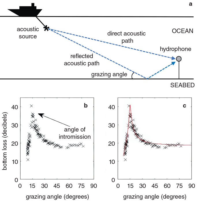
A useful remote-sensing method for estimating mud sound speeds and other properties involves what are called seabed reflection coefficients. The measurement procedure is illustrated in the figure above. A hydrophone (or underwater microphone) is used to record acoustic pulses from an acoustic source that follow direct and bottom-reflected paths through the water column. The reflection coefficient is defined as the ratio of the reflected wave acoustic pressure to that of the direct wave, and thus quantifies how the reflection process has altered the wave amplitude. Measuring reflection coefficients for a range of angles using a towed acoustic source provides a dataset that contains a great deal of information about seabed geoacoustic properties.
A particularly interesting case involves data with what is called an angle of intromission, that is, an angle at which the reflection coefficient goes to zero and there is no reflected acoustic wave but rather total transmission into the seabed. The angle of intromission was predicted theoretically by English scientist Lord Rayleigh in 1896. Rayleigh showed that the angle of intromission exists for reflection at the interface between two media with sound speed and density ratios less than and greater than 1, respectively.
Because muds often have a sediment sound speed ratio less than 1 and always have a density ratio greater than 1, an angle of intromission should commonly occur in seabed acoustic-reflection measurements. However, there have been only a few successful field measurements of this occurrence. One reason is that it is challenging to measure the absence of something—in this case, the reflected field. Not only does the signal-to-noise ratio have to be high, but all other “contaminating” paths must be mitigated, including reflected waves from deeper layers in the seabed.
The first clear angle of intromission measurement was published in 1968 by Robert S. Winokur and Joyce C. Bohn of the U.S. Naval Oceanographic Office, who found an angle of intromission of 11 degrees in a deep-ocean setting, with a water depth of 4,500 meters. The next observation came more than three decades later in 2002, when one of us (Holland) measured an angle of intromission of 15 degrees in 100 meters of water at several sites in Italian coastal waters. One of these datasets is shown in the figure above, in terms of bottom loss in decibels (with high bottom loss corresponding to low reflection coefficients), clearly showing the angle of intromission.
Using measurements of the angle of intromission and bottom loss at one other angle, the seabed sound speed and density can be calculated from Lord Rayleigh’s theories, with values of 1,480 ± 4 meters per second (with a sediment sound speed ratio of 0.979 ± 0.003) and 1.32 ± 0.04 grams per cubic centimeter, respectively, at this site. Using those geoacoustic estimates, the full bottom loss can be calculated theoretically, which compares closely with the measured data. These data, collected south of Sicily, have the same angle of intromission as data at the same water depth 1,000 kilometers away, north of the island of Elba in Italy in the Tyrrhenian Sea. This result suggests that the physical processes that govern the mud microstructure are likely similar at the two sites.
The approach given above estimated depth-independent mud geoacoustic parameters using the angle of intromission at a single frequency. But what if the angle of intromission is observed to be frequency dependent? It is well-known that the acoustic penetration depth in sediment decreases with frequency (or increases with wavelength) such that very high frequencies (or short wavelengths) are sensitive only to near-surface geoacoustic properties, whereas low frequencies (or long wavelengths) are sensitive to deeper properties. Thus, depth-dependent sound speed and density profiles lead to a frequency-dependent angle of intromission.
Conversely, frequency-dependent angle of intromission observations provide information about, and can be inverted for, geoacoustic profiles. We formulated a Bayesian (or probabilistic) inversion of measured bottom loss data to estimate sound speed and density profiles. The results show the most probable depth-dependent sound speed and density profiles with uncertainties (see figure below).
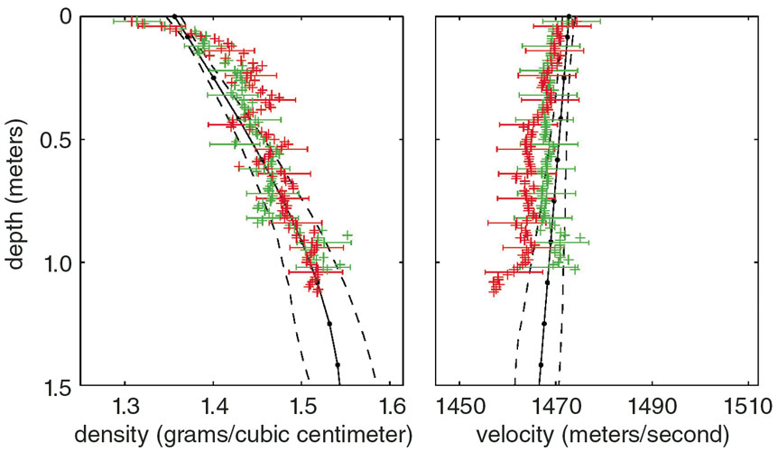
C. W. Holland et al., 2005.
This figure also shows depth-dependent geoacoustic properties measured from two cores collected at the site, using specially designed corers to minimize sediment disturbance, which revealed the mud to be a nannofossil ooze. The agreement between the geoacoustic properties estimated remotely via angle of intromission inversion and the core measurements is generally quite good, with a sediment sound speed ratio of 0.976. It is clear that the angle of intromission frequency dependence does contain significant information about the depth dependence of the mud properties.
A simple theory that takes the weighted average of the water and the mud particle component properties predicts that the minimum possible sediment sound speed ratio value for mud is about 0.97. In other words, the minimum sound speed in mud is about 3 percent lower than that in seawater. Measurements over the past decades confirm this minimum value for muddy sediments with seawater in the interstices (although occasionally, the presence of gas bubbles rather than water in muds can reduce the sound speed much more).
A few percent variation in sound speed may seem hardly worth noting, but for ocean acoustic propagation, the effect can be considerable. In continental shelf areas, sound can travel long distances because of the formation of what’s called an acoustic waveguide between the sea surface and the seabed, given suitable seabed properties. For example, with sandy sediments, the sound speed is greater than that of water (so the sediment sound speed ratio is greater than 1), and a critical reflection angle exists at which the acoustic wave is completely reflected with no acoustic transmission into the seabed (typically at a 15 to 30 degree grazing angle). In such cases, acoustic energy can propagate at angles below the critical angle with little loss over very long distances, equivalent to hundreds of times the depth of the water.
However, for a muddy sediment with a sediment sound speed ratio below 1, no critical angle (and therefore no acoustic waveguide) exists. Put another way, for a sediment with a sediment sound speed ratio below 1, sound propagation in the ocean is limited to distances equivalent to only a few water depths. However, this occurrence rarely happens in practice at frequencies below 10 kilohertz for two main reasons. First, mud generally has a very low attenuation, compared with sand. Thus, even for a mud layer tens of meters thick overlying sand, an acoustic waveguide often exists between the sea surface and the buried sand layer. Second, the mud sound speed can increase with depth such that there is a turning point within the mud where refraction bends the sound waves upward, returning acoustic energy to the water column. This event occurs often in deep-water environments where muddy sediments can be many kilometers thick. Both reasons underscore the importance of understanding the depth dependence of sediment geoacoustic properties.
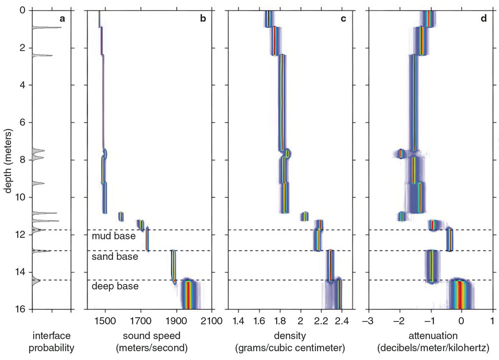
At the New England Mud Patch, depth-dependent mud properties were inferred using reflection-coefficient data and Bayesian geoacoustic inversion, a statistical method to reconstruct the inputs or parameters that produced an observed effect. The results are shown in the figure below, plotted in terms of probability profiles for geoacoustic parameters. At this site, the mud thickness is found to be about 11.7 meters. As is the case across the New England Mud Patch experimental area, a sand layer exists below the mud. The mud geoacoustic properties appear to fall into three depth intervals: upper 0–3 meters, middle 3–10.8 meters, and lower 10.8–11.7 meters. The sound speed increases with depth in the upper interval, is nearly uniform in the middle, and exhibits an extremely large gradient in the lower.
When first observed, the high gradients in the lower mud interval were puzzling, but have since been determined to arise from sand particles from the sand layer below the mud that were entrained in the mud at the time the mud began to be deposited at the end of the last glaciation, about 10,000 years ago. Charles Nittrouer of the State University of New York at Stony Brook and his colleagues found in 1986 that biologic processes aided this entrainment, and John A. Goff of the University of Texas at Austin and his colleagues in 2019 identified geologic processes that also contributed. The fraction of sand increases with depth in the interval, which leads to the increase in sound speed. We term this lower interval the transition interval because it represents a gradual transition from mud to sand, as opposed to a sudden change in sediment type.
Geoacoustic inversion results at two other sites at the New England Mud Patch—at 5 kilometers and 19 kilometers to the northwest, with mud thicknesses of 10 meters and 3 meters, respectively—show remarkable similarity in the transition interval, its thickness, and sound speed gradient. This finding suggests that the geologic and biologic processes contributing to its formation were fairly uniform across the mud patch during the formation time. The other two sites also show similar depth dependence in the upper and middle intervals.
Attenuation is a challenging property to determine in sediments. Nevertheless, the inferred attenuation for the New England Mud Patch data (see figure below) is sufficiently well determined and has small enough uncertainties that we can discern its variation with depth. In the upper interval, attenuation decreases exponentially with depth (linearly in the log plot, smoothing through the stairsteps), is roughly constant in the middle interval, and increases rapidly in the lower (transition) interval. The large attenuation increase in the transition interval—nearly two orders of magnitude—is known to be due to the increasing sand content. At the two other sites at the New England Mud Patch (5 and 19 kilometers away), the attenuation exhibits a similar depth dependence. Recent core data at several locations near the site also show an exponentially decreasing attenuation in the upper layer at frequencies in the low hundreds of kilohertz.
Y.-M. Jiang et al., 2023.
The transition interval is controlled by biologic processes (such as mixing by bottom-dwelling fauna) and geologic processes (such as sea-level oscillations and sediment transport from storms). Because these processes are virtually ubiquitous across the planet, it seems likely that the transition interval may exist at all or at least at many, muddy continental shelves. The characteristics of the transition interval are expected to vary depending on the regional processes. However, transition-interval characteristics may be approximately spatially uniform for a given shelf region. The transition interval and its similarity in a given region have been observed for the two continental shelf regions studied thus far in the North Atlantic and the Mediterranean. Thus, if sediment mixing and mud deposition rates are known for a given shelf, it may be possible to predict the transition interval thickness and geoacoustic characteristics and, hence, make better predictions of the depth-averaged attenuation in the mud layer. With improved geoacoustic properties, better predictions of the acoustic field in the ocean can be made, improving our ability to operate in and understand the ocean.
The frequency dependencies of the sound speed and especially attenuation are important to understanding ocean-acoustic propagation in a particular environment. In theory, the attenuation can increase with frequency at rates varying from frequency to the one-half power to frequency squared, but the actual form of the frequency dependence for specific sediments is difficult to measure accurately. Nonetheless, it’s quite important to measure because the change in attenuation with frequency over a few octaves can be dramatic.
There is growing evidence at the New England Mud Patch and other areas that muds with a modest sand content follow a nearly linear dependence of attenuation on frequency above a few tens of hertz up to at least 10 kilohertz. Furthermore, several observations, such as those made in 2020 by Jie Yang and Darrell Jackson of the University of Washington, have demonstrated that mud sound speed shows little variation with frequency from a few tens of hertz to hundreds of kilohertz. However, it should be noted that there are numerous other measurements of mud sound speed and attenuation, and there is not yet consensus as to the frequency and depth dependence of mud, even in the well-studied New England Mud Patch.
Sediment-acoustic models are crucial for advancing our understanding of mud acoustics. These models predict wave speeds and attenuations as a function of frequency from a set of physical properties such as porosity. Carrying out geoacoustic measurements can be expensive, and if only a single measurement is available, say a core at 100 kilohertz, but a specific application requires a sound speed or attenuation at 100 hertz, models are required to bridge the spectral gap. More fundamentally, models provide a framework to test hypotheses and provide important constraints—for example, that the frequency dependencies of sound speed and attenuation are linked as a consequence of causality. Geoacoustic measurements and inferences, in turn, guide model development by providing observables that yield clues about the important underlying physics. Three sediment-acoustic models are currently used for muds; two of them have origins in models of wave propagation in granular media, and the third was developed specifically for mud.
The first model is based on theories by Belgian-American physicist Maurice A. Biot from the early 1960s. This model, proposed in 2021 by Nicholas Chotiros of the University of Texas at Austin and his colleagues, is known as the mCREB model (for modified, corrected, Revil, extended Biot; Revil refers to geophysicist André Revil of the University of Savoy in France, who has also done theoretical work in this area). Biot’s original pioneering work involved modeling wave propagation through consolidated but porous media, such as rocks. This theory was subsequently modified over time to treat unconsolidated sediments. Most of the numerous subsequent Biot theory variants have been aimed at sands and silts, but a few treat mud. This most recent mud variant, mCREB, includes the mechanism of fluid flow at grain-to-grain contacts that was developed for granular media, and adds mechanisms believed to be important for mud, including electrochemical forces binding a thin film of pore water to grain surfaces, the presence of tiny grains suspended in the pore water, and a mechanical process called creep, in which the material strain in the mud continues to increase under a constant stress.
Finally, the silt-suspension theory (SST) was developed by Allan D. Pierce of the Cape Cod Institute for Science and Engineering and his colleagues in 2017. It considers mud composed of silt grains suspended in an effective fluid consisting of water and a matrix of clay particles. The clay particles are assumed to be arranged in a so-called cardhouse structure, formed because the clay particles are electrically charged and can stick together face-to-edge, much like a house of cards. Whereas mCREB and VGS are phenomenological models, SST attempts to work from the first principles of basic physical quantities, including the electrostatic forces for clay and the classical Stokes theory—which determines frictional forces on tiny spherical objects—for the suspended silt. More recent work has invoked a continuous smear of relaxation processes (in which a perturbed material returns to its original, undisturbed state) that can be associated with diverse types of solid particles nominally in contact, but sliding and separating in acoustic wave propagation.
Similarities exist between these models: Strain hardening, creep, and relaxation processes are related. Differences also exist, of course, as evidenced by the differences in frequency dependencies predicted by the various models.
There is still a lively debate about the properties of marine muds, including their depth and frequency dependencies. Furthermore, challenges remain in reconciling remote measurements with one another, direct measurements with one another, remote and direct measurements, and measurements with models.
We still don’t know whether mud properties vary with seasonal changes in seawater temperature.
Outstanding questions are being actively pursued in mud acoustics research. For instance, researchers are trying to determine what the key geologic, biologic, and chemical processes are that lead to vertical and lateral variations in the geoacoustic properties of muds. Furthermore, what generalizations can be made for extrapolating findings for one muddy environment to other locations and mud types around the world? And we still don’t know whether mud properties vary over time, for example, with seasonal changes in the seawater temperature.
But we do know that characterizing the Earth’s oceans accurately is key to understanding them, especially as our planet continues to change over time, and we won’t be able to achieve this goal without a clearer understanding of mud.
This article is adapted from Acoustics Today 20:37–45 with permission from the Acoustical Society of America.
Click "American Scientist" to access home page

American Scientist Comments and Discussion
To discuss our articles or comment on them, please share them and tag American Scientist on social media platforms. Here are links to our profiles on Twitter, Facebook, and LinkedIn.
If we re-share your post, we will moderate comments/discussion following our comments policy.