American Scientist

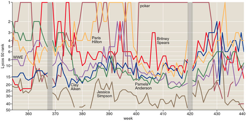
Back in 1999, the operators of the Lycos Internet portal began publishing a weekly list of the 50 most popular queries submitted to their Web search engine. Britney Spears—initially tagged a "teen songstress," later a "pop tart"—was No. 2 on that first weekly tabulation. She has never fallen off the list since then—440 consecutive appearances when I last checked. Other perennials include ­Pamela Anderson and Paris Hilton. What explains the enduring popularity of these celebrities, so famous for being famous? That's a fascinating question, and the answer would doubtless tell us something deep about modern culture. But it's not the question I'm going to take up here. What I'm trying to understand is how we can know Britney's ranking from week to week. How are all those queries counted and categorized? What algorithm tallies them up to see which terms are the most frequent?

One challenging aspect of this task is simply coping with the volume of data. Lycos reports processing 12 million queries a day, and other search engines, such as Google, handle orders of magnitude more. But that's only part of the problem. After all, if you have the computational infrastructure to answer all those questions about Britney and Pamela and Paris, then it doesn't seem like much of an added burden to update a counter each time some fan submits a request. What makes the counting difficult is that you can't just pay attention to a few popular subjects, because you can't know in advance which ones are going to rank near the top. To be certain of catching every new trend as it unfolds, you have to monitor all the incoming queries—and their variety is unbounded.

In the past few years the tracking of hot topics has itself become a hot topic in computer science. Algorithms for such tasks have a distinctive feature: They operate on a continuous and unending stream of data, rather than waiting for a complete batch of information to be assembled. Like a worker tending a conveyor belt, the algorithm has to process each element of the stream in sequence, as soon as it arrives. Ideally, all computations on one element are finished before the next item comes along.

Much of the new interest in stream algorithms is inspired by the Internet, where streams of many kinds flow copiously. It's not just a matter of search-engine popularity contests. A similar algorithm can help a network manager monitor traffic patterns, revealing which sites are generating most of the volume. The routers and switches that actually direct the traffic also rely on stream algorithms, passing along each packet of data before turning to the next. A little farther afield, services that filter spam from e-mail can use stream algorithms to detect messages sent in thousands or millions of identical copies.

Apart from the Internet, stream algorithms are also being applied to flows of financial data, such as stock-market transactions and credit-card purchases. If some government agency wanted to monitor large numbers of telephone calls, they too might have an interest in stream algorithms. Finally, the designers of software for some large-scale scientific experiments adopt a stream-oriented style of data processing. Detectors at particle-physics laboratories produce so much data that no machine can store it all, even temporarily, and so preliminary filtering is done by programs that analyze signals on the fly.

Stream Gauges

Search-engine queries and Internet packets are fairly complicated data structures, but the principles of stream algorithms can be illustrated with simple streams of numbers. Suppose a pipeline delivers an endless sequence of nonnegative integers at a steady rate of one number every t time units. We want to build a device—call it a stream gauge—that intercepts the stream and displays answers to certain questions about the numbers.

What computational resources does a stream gauge need to accomplish its task? The resources of particular concern are processing time—which can't exceed t units per stream element—and auxiliary storage space. (It's convenient to assume that numbers of any size can be stored in one unit of space, and that any operation of ordinary arithmetic, such as addition or multiplication, can be performed in one unit of time. Comparing two numbers also takes a single time unit.)

For some questions about number streams, it's quite easy to design an effective stream gauge. If you want to know how many stream elements have been received, all you need is a counter. The counter is a storage location, or register, whose initial value is set to 0. Each time an ele­ment of the stream arrives, the counter is incremented: In other words, if the current value of the counter is x , it becomes x +1.

Instead of counting the stream elements, another kind of gauge displays the sum of all the integers received. Again we need a register x initialized to 0; then, on the arrival of each integer n , we add n to the running total in x .

Still another easy-to-build gauge shows the maximum value of all the integers seen so far. Yet again x begins at 0; whenever a stream element n is greater than x , that n becomes the new x .

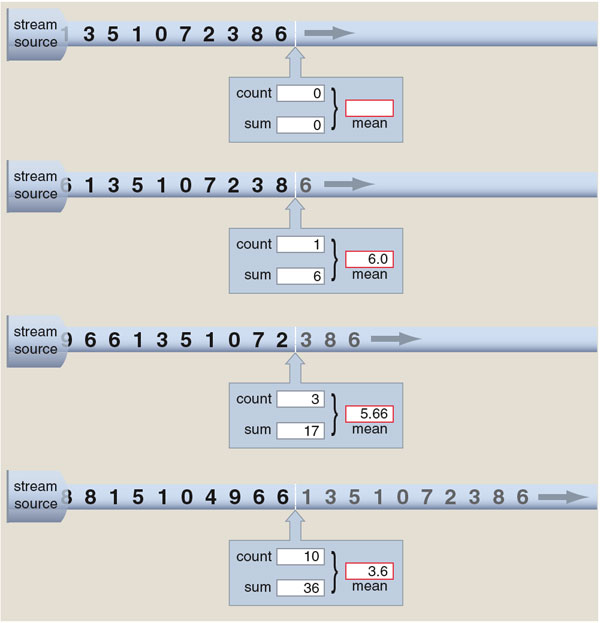
For each of these devices, the storage requirement is just a single register, and the processing of each stream element is completed in a single unit of time. Computing doesn't get much easier than that. Certain other stream functions require only slightly greater effort. For example, calculating the average (or arithmetic mean) of a stream's integers takes three registers and three operations per integer. One register counts the elements, another records their sum, and the third register holds the value of the average, calculated as the quotient of the sum and the count.

What matters most about the frugal memory consumption of these algorithms is not the exact number of registers needed; what matters is that the storage space remains constant no matter how long the stream. In effect, the algorithms can do calculations of any length on a single sheet of scratch paper. Their time performance follows a similar rule: They use the same number of clock cycles for each element of the stream. The algorithms are said to run in constant space and constant time.

Logjam

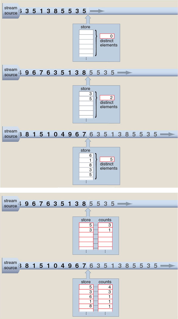
Not every property of a stream can be computed in constant space and time. Consider a device that reports the number of distinct elements in a stream of integers. (For example, although the stream 3, 1, 8, 3, 1, 4, 3 has a total of seven elements, it has only four distinct elements: 3, 1, 8 and 4.)

There's a straightforward method for counting distinct elements: Start a counter at 0 and increment the counter whenever the stream delivers a number you haven't seen before. But how do you know that a given number is making its first appearance? The obvious answer is to keep a list of all the integers you've encountered so far, and compare each incoming value n with the numbers in the stored set. If n is already present in the list, ignore the new copy. If n is not found, append it to the stored set and increment the counter.

The trouble is, this is not a constant-space algorithm. The set of stored values can grow without limit. In the worst case—where every element of the stream is unique—the size of the stored set is equal to the length of the stream. No fixed amount of memory can satisfy this appetite.

The problem of counting distinct elements is closely related to the problem of identifying the most-frequent elements in a stream. Having a solution to one problem gives us a head start on the other. The distinct-elements algorithm needs to keep a list indicating which stream elements have been observed so far. The frequent-elements algorithm needs the same list, but instead of simply noting whether or not an element is present, the program must maintain a counter for each element, giving its frequency. Since the list of elements and their counters can grow without limit, demands for space are again potentially unbounded.

Both of the algorithms could run out of time as well as space, depending on details of implementation. If it's necessary to search through all the stored numbers one by one for every newly received stream element, then the time needed grows in proportion to the size of the stored set. Eventually, the delay must exceed t , the interval between stream elements, at which point the algorithm can no longer keep up with the incoming data. Other data structures, such as trees and indexed arrays, allow for quicker access, although other time constraints may remain.

Majority Rules

Stream algorithms that require more than a constant amount of storage space are seldom of practical use in large-scale applications. Unfortunately, for tasks such as counting distinct elements and finding most-frequent elements, there is really no hope of creating a constant-space algorithm that's guaranteed always to give the correct answer. But before we grow too despondent about this bleak outlook, I should point out that there are also a few pleasant surprises in the world of stream algorithms.

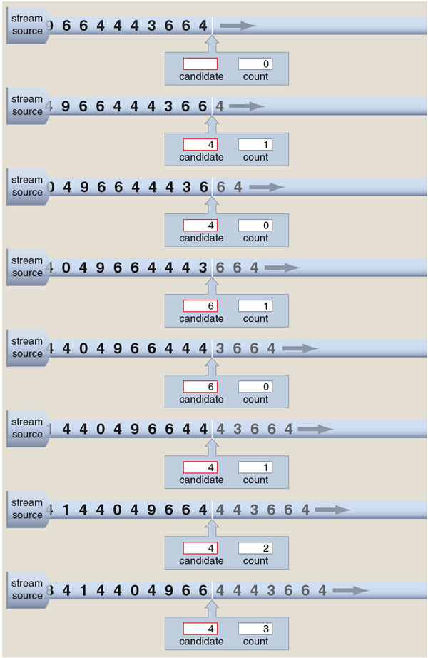
Although identifying the most frequent item in a stream is hard in general, there is an ingenious way of doing it in one special case—namely, when the most common item is so popular that it accounts for a majority of the stream entries (more than half the elements). The algorithm that accomplishes this task requires just two registers, and it runs in a constant amount of time per stream element. (Before reading on you might want to try constructing such an algorithm for yourself.)

The majority-finding algorithm uses one of its registers for temporary storage of a single item from the stream; this item is the current candidate for majority element. The second register is a counter initialized to 0. For each element of the stream, we ask the algorithm to perform the following routine. If the counter reads 0, install the current stream element as the new majority candidate (displacing any other element that might already be in the register). Then, if the current element matches the majority candidate, increment the counter; otherwise, decrement the counter. At this point in the cycle, if the part of the stream seen so far has a majority element, that element is in the candidate register, and the counter holds a value greater than 0. What if there is no majority ele­ment? Without making a second pass through the data—which isn't possible in a stream environment—the algorithm cannot always give an unambiguous answer in this circumstance. It merely promises to correctly identify the majority element if there is one.

The majority algorithm was invented in 1982 by Michael E. Fischer and Steven L. Salzberg of Yale University. The version I have described here comes from a 2002 article by Erik D. Demaine of MIT and Alejandro López-Ortiz and J. Ian Munro of the University of Waterloo in Canada. Demaine and his colleagues have extended the algorithm to cover a more-general problem: Given a stream of length n, identify a set of size m that includes all the elements occurring with a frequency greater than n /( m +1). (In the case of m =1, this reduces to the majority problem.) The extended algorithm requires m registers for the candidate elements as well as m counters. The basic scheme of operation is analogous to that of the majority algorithm. When a stream ele­ment matches one of the candidates, the corresponding counter is incremented; when there is no match to any candidate, all of the counters are decremented; if a counter is at 0, the associated candidate is replaced by a new element from the stream.

Again the results carry only a weak guarantee: If any elements of the stream exceed the threshold frequency, those elements will appear among the candidates, but not all the candidates are necessarily above the threshold. Even with this drawback, the algorithm performs impressive feats, such as scanning a stream of Web search queries for all terms that make up at least 1 percent of the traffic.

Getting It Almost Right

For many stream problems of practical interest, computing exact answers is simply not feasible—but it's also not necessary. A good estimate, or an answer that's probably correct, will serve just fine.

One simple approach to approximation is to break a stream into blocks, turning a continuous process into a series of batch operations. Within a block, you are not limited to algorithms that obey the one-pass-only rule. On the other hand, answers derived from a sequence of blocks only approximate answers for the stream as a whole. For example, in a count of distinct elements, an item counted in two successive blocks would be counted only once if the blocks were combined.

A variant of the block idea is the sliding window. A window of length k holds the most recent k elements from the stream, with each new arrival displacing the oldest item in the queue.

A great deal of ingenuity has been applied to the search for better approximate stream algorithms, and there are successes to report. Here I shall briefly mention work in two areas, based on sampling and on hashing.

When the items that interest you are the most frequent ones in a stream, statistics is on your side; any sample drawn from the stream is most likely to include those very items. Indeed, any random sample represents an approximate solution to the most-common-elements problem. But the simplest sampling strategy is not necessarily the most efficient or the most accurate. In 2002 Gurmeet Singh Manku and Rajeev Motwani of Stanford University described two methods they called sticky sampling and lossy counting.

Suppose you want to select a representative sample of 100 items from a stream. If the stream consists of just 100 elements, the task is easy: Take all the elements, or in other words select them with probability 1. When the stream extends to 200 elements, you can make a new random selection with probability 1/2; at 400 elements, the correct probability is 1/4, and so on. Manku and Motwani propose a scheme for continually readjusting the selection probability without having to start over with a new sample. Their sticky-sampling method refines the selection each time the stream doubles in length, maintaining counters that estimate how often each item appears in the full stream. The algorithm solves the most-frequent-elements problem in constant space, but only in a probabilistic sense. If you run the algorithm twice on the same data, the results will likely differ.

Lossy counting is based on a similar idea of continually refining a sample as the stream lengthens, but in this case the algorithm is deterministic, making no use of random choices. Each stream element is checked against a stored list; if the element is already present, a counter is incremented; otherwise a new entry is added. To keep the list from growing uncontrollably, it is periodically purged of infrequent elements. Lossy counting is not guaranteed to run in constant space, but Manku and Motwani report that in practice it performs better than sticky sampling.

Making A Hash of It

Hashing—one of the more aptly named techniques of computer science—is a way of scrambling data so that the result looks random. Oddly enough, this turns out to be a good way of making sense of the data.

A completely random stream might seem hard to analyze, but in fact randomness opens the door to some simple but powerful statistical methods. Imagine a stream composed of numbers chosen at random from some fixed range of integers, say 1 through n . For this stream the number of distinct elements observed follows a highly predictable course; in particular, all n distinct elements should have appeared at least once by the time the stream reaches length n log n.

This kind of analysis won't work for most streams of real data because the elements are not drawn from a convenient fixed range, and they are not random—unless you compose search-engine queries by blindly pecking at the keyboard. This is where hashing comes in. A hash function transforms a data item into a more-or-less random value uniformly distributed over some interval. Think of hashing as the action of a mad postal clerk sorting letters into bins. The clerk's rule says that if two letters have the same address, they go into the same bin, but in all other respects the sorting might as well be random.

By randomly distributing all the elements of a stream into a fixed number of bins, hashing allows for easy statistical analysis of the stream's elements. For example, the number of distinct elements can be estimated from the probability that a given bin remains empty, or from the minimum number of elements found in any bin. A recent paper by Ahmed Metwally and Divya­kant Agrawal of Ask.com and Amr El Abbadi of the University of California, Santa Barbara, evaluates a dozen of these algorithms.

Gently Down the Stream

Are there better algorithms for stream problems waiting to be discovered? Some of the limits of what's possible were outlined in 1996 by Noga Alon, Yossi Matias and Mario Szegedy, who were all then at AT&T Bell Laboratories. They framed the issue in terms of an infinite series of frequency moments , analogous to the more familiar statistical moments (mean, variance, and so on). The zero-order frequency moment F ₀ is the number of distinct elements in the stream; the first-order moment F ₁ is the total number of elements; F ₂ is a quantity called the repeat rate; still higher moments describe the "skew" of the stream, giving greater emphasis to the most-frequent elements. All of the frequency moments are defined as sums of powers of m _i , where m _i is the number of times that item i appears in a stream, and the sum is taken over all possible values of i .

It's interesting that calculating F ₁ is so easy. We can determine the exact length of a stream with a simple, deterministic algorithm that runs in constant space. Alon, Matias and Szegedy proved that no such algorithm exists for any other frequency moment. We can get an exact value of F ₀ (the number of distinct elements) only by supplying much more memory. Even approximating F ₀ in constant space is harder: It requires a nondeterministic algorithm, one that makes essential use of randomness. The same is true of F ₂ . For the higher moments, F ₆ and above, there are no constant-space methods at all.

All this mathematics and algorithmic engineering seems like a lot of work just for following the exploits of a famous "pop tart." But I like to think the effort might be justified. Years from now, someone will type "Britney Spears" into a search engine and will stumble upon this article listed among the results. Perhaps then a curious reader will be led into new lines of inquiry.