Knowledge Discovery and Data Mining
By Carla Brodley, Terran Lane, Timothy Stough
Computers taught to discern patterns, detect anomalies and apply decision algorithms can help secure computer systems and find volcanoes on Venus
Computers taught to discern patterns, detect anomalies and apply decision algorithms can help secure computer systems and find volcanoes on Venus

DOI: 10.1511/1999.16.54
One of the most important parts of a scientist's work is the discovery of patterns in data. Yet the databases of modern science are frequently so immense that they preclude direct human analysis. Inevitably, as their methods for gathering data have become automated, scientists have begun to search for ways to automate its analysis as well.
Over the past five years, investigators in a new field called knowledge discovery and data mining have had notable successes in training computers to do what was once a unique activity of the human brain.
The study of climate change provides an excellent example of the difficulties of extracting useful information from modern databases. In recent years, many questions about the earth's climate have moved into the realm of public policy: How rapidly are we destroying tropical rain forests? Is the Sahara Desert growing? What might be the effects of global warming, and has it started already?
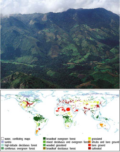
Aerial photograph courtesy of Doug Muchoney, Center for Remote Sensing, Boston University; map image courtesy of Ruth DeFries, University of Maryland, and John Hodges, Boston University.
An important factor in any climate model is the distribution of different kinds of vegetative land cover. Plants play a huge and so far not completely understood role in moderating the earth's carbon cycle, including the levels of carbon dioxide in the atmosphere. Since the late 1970s, climatologists have been able to follow changes in global land cover by satellite, but the instruments they use were not really designed for that purpose. That will change next year, when NASA is scheduled to launch a new satellite network devoted exclusively to earth science, the Earth Observing System (EOS). But with greater opportunity comes greater challenge. EOS is expected to gather 46 megabytes of data per second; a single day's data will require the space it would take to store 1,500 copies of the 32-volume text of the Encyclopaedia Britannica. Such a volume of information threatens to overwhelm many of the tools available to analyze it.
Nor is sheer volume the only problem. To make sense of the satellite data, analysts will have to correlate it with existing global vegetation maps. These maps, produced by direct observation on the ground as well as by prediction of "potential vegetation" (the vegetation that is natural to a region given its climate and latitude), disagree with each other to an amazing extent. When they compared three reference maps, geographers Ruth DeFries and John Townshend of the University of Maryland found that they agreed on roughly 20 percent of the earth's land surface. One map's grasslands are another map's badlands.
A third problem is that of interpretation. If a particular pixel in the satellite data is "green" in January and again in June, does that mean the pixel represents a tropical rainforest? And just how "green" does it have to be? Some rules may be part of the existing base of scientific knowledge, but others may be hidden in the data and awaiting discovery. In applications of data mining to other sciences, even the relevant categories—the equivalent of "grassland" or "tropical rain forest"—may be unknown.
Because it offers a way to detect patterns in large and messy data sets, data mining has become fashionable in a very short time, especially in the business world. We shall present applications that range from finding volcanoes on Venus to making printing presses run better, and explain one of the more popular data-mining methods, called "decision trees." First we offer as a caveat one lesson we have learned along the way: However tempting it may seem to leave everything to the computer, knowledge discovery is still a collaborative process that involves human expertise in a fundamental way.
Data mining is just one part of the process of knowledge discovery in data bases (often abbreviated KDD). KDD is an iterative process with six stages: 1) develop an understanding of the proposed application; 2) create a target data set; 3) remove or correct corrupted data; 4) apply data-reduction algorithms; 5) apply a data-mining algorithm; and 6) interpret the mined patterns. Some steps may be skipped, and the process is not necessarily sequential—often the results of one step cause the practitioner to back up to an earlier one. Although research tends to focus on step 5, the steps before and after data mining are equally important. In particular, it takes an expert in the application field, not a KDD expert, to decide whether the mined patterns are meaningful.
When we began to work on the global land-cover problem, we first determined 12 categories of interest: tundra, wooded grassland and so forth. The satellites that provided our data could not count trees or tell grass apart from crops; they could only measure the reflectivity of the surface at certain wavelengths and at certain times of the year. Thus our data-mining objective was to come up with rules for converting those measurements to an appropriate land-cover category for each pixel in our world map.
After we defined the problem, the next step was the creation of training data. This is a subset of the data that trains the data-mining algorithm to interpret the rest of the data correctly—just as a student learns a new subject by solving practice problems. Sometimes the KDD system itself can identify useful portions of the data for training; other times, a domain expert (human or not) performs this task. In our case, we selected only pixels where three existing vegetation maps agreed. In effect, we used the consensus of the three maps as our domain expert.
The choice of training examples is both an important and an extremely challenging task. The sample must be large enough to justify the validity of the discovered knowledge. Otherwise, like a student who has done too few practice problems, the data-mining program is likely to discover "rules" that don't work on other parts of the data. (Because of the low quality of the output, mining small data sets is sometimes called "data dredging.")
After selecting the training data, the next step is to clean the data and select or enhance the relevant features. For example, in a business application a person's income might be relevant to marketing strategies, but his or her Social Security number would not. Data reduction through feature enhancement is particularly important in image databases because of the sheer magnitude of the pixel data. We shall describe this below, in the context of our project to identify volcanoes on Venus.
Linda Huff
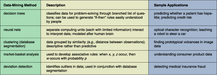
Next comes the choice of a data-mining algorithm. There are myriad methods available, and the choice depends strongly on the kind of data and the intended use for the mined knowledge. Is the model intended to be predictive or explanatory? Should the patterns discovered be understandable by people, or is reliability the most important consideration? Neural networks, for example, have been very popular in the machine learning community—they have been used to create machines that can recognize barcodes or learn to steer a car. But they are often less suitable for KDD, because they do not explain to a human user how they arrive at their predictions. If the goal of knowledge discovery is human knowledge, a "black box" oracle cannot be a desirable solution.
For the land-cover data we chose a decision-tree algorithm, because it produces a classification structure that is particularly easy for a person to understand. Decision trees have had many business and industrial applications; for example, in the financial industry, they are used to decide whether a person is a good or poor credit risk. We shall explain below what a decision tree is and how a decision-tree algorithm finds it.
Knowledge discovery does not end with the data-mining algorithm. The remaining step is to interpret the meaning of the mined patterns and verify that they are accurate. The interpretation can often be assisted by visualization methods, another large field of research. (See Brown et al. 1995 for an introduction.) Accuracy can be assessed by testing the results on a set of validation data. If the decision tree does not perform well enough, or if nothing of interest has been found, the investigator must go back to a previous step. In the land-cover example, our decision tree predicted the correct type of vegetation over 90 percent of the time, making the results reliable enough to use in climatology models.
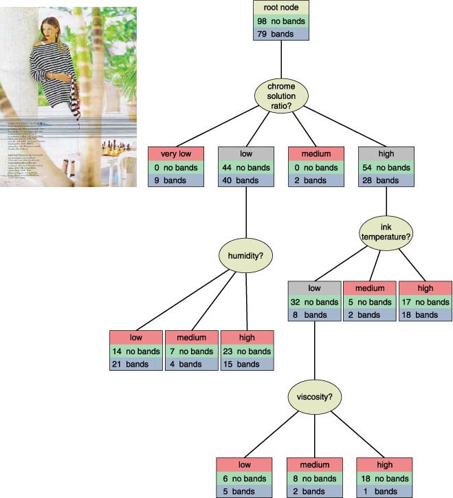
For years, rotogravure printing presses have been plagued by a sporadic problem known as "banding." Rotogravure banding takes place when grooves become engraved onto a cylinder surface, and it shows up as a line of ink across pages of printed matter. The printing company RR Donnelley and Sons applied a decision-tree algorithm to discover the cause. Robert Evans, a technology specialist at RR Donnelley, collected machine data from printer operations, both under normal conditions and when banding occurred. The database from which he and Doug Fisher of Vanderbilt University built the decision tree eventually consisted of measurements on 30 different attributes during approximately 500 press runs—250 when banding did not occur and 250 when it did.
Aaron Cox
Figure 3 shows a subtree of the decision tree that Evans and Fisher constructed. Out of the 30 variables measured, they found that the most predictive was the chrome solution ratio—the proportion of chrome in the plating solution, used to extend the life of the printing plates. When it was "very low" (actual numbers are not given, as they are proprietary to Donnelley), banding always occurred. But banding was also seen sometimes when the chrome solution ratio was "low" or "high," so the algorithm added further branches to the decision tree to identify other risk factors in these cases. Because the decision tree produced rules that could be put into operation, Donnelley was able to reduce the incidence of banding from 538 occurrences in 1989 to 37 in 1997.
As this example shows, a decision tree is essentially a branched list of questions in which the answer to one question determines the next question asked. Each question is called a "node" on the tree, and each answer leads to a separate "branch." At the end of each branch lies a "leaf node," where the decision tree assigns a classification to the data. For example, at the leaf node "very low chrome solution ratio," the model predicts a high risk of banding; at the leaf node "high chrome ratio/low ink temperature/high viscosity," it predicts a low risk. The more clear-cut the classification at each leaf node, the better; but, as this example shows, the data may not allow for a perfect split.
The decision subtree in Figure 3 is fairly simple, with only four test questions and ten leaf nodes. In general, a tree will be larger if there are more categories to separate the data into, or if more complex decision procedures are required. Evans and Fisher had only two categories (banding/no banding). In the land-cover problem, which had 12 categories, our decision tree had 120 questions and 121 leaf nodes. Of course, only a small fraction of these questions would be required to classify any particular pixel.
How, then, does a computer find the right decision tree? The answer is a combination of brute-force search and information theory.
As we have seen, a decision tree is generated from a set of training data, which we can call D. (Initially, D would be the whole training data set; at later steps, it represents only a part of the training data.) Each observation in D has been assigned by an expert to one of several categories, which we denote by C1, C2 and so on. The job of the decision tree is to reproduce this assignment as accurately as possible.
Each node of the decision tree contains a test or splitting rule T. In the simplest case, this is a yes-no question. It splits the data into two mutually exclusive subsets: the observations for which the answer to the question is "yes" and the observations for which the answer is "no." The best test question would be one for which all of the "yes" (or all of the "no") observations fell into one category Ci. (For example, in the printing-press data, when the answer to "Is the chrome solution ratio very low?" was "yes," banding was always observed.) More often, no single test will be able to make such a clear-cut classification at the top of the decision tree. In that case, the decision-tree algorithm looks for the best available test—the one that makes the most progress toward the correct classification. This part is typically done by brute force, simply by considering every possible test. But a crucial question arises: How do we measure "progress" toward our goal? This measurement is the most important element of a decision-tree algorithm.
Aaron Cox
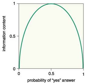
To measure how good a test is, we can recall the game of Twenty Questions, in which one player asks yes-no questions of the other player ("is it bigger than a breadbox?") in order to identify some object in the room. If we consider the set of possible objects to be of fixed size, then we are interested in answering the following questions: Given a set S (whose number of elements is denoted |S|) and the ability to ask yes-no questions about a particular element of the set x, what is the minimum number of questions you need to ask, in the worst case, to determine what x is?
The answer is log2|S|, because the best we can do at each point is split the data in half. Note that we could get a 30/70 split and with luck get into the 30 split; that is, we could immediately identify the object as part of a minority subset, sharply reducing the remaining possibilities. However, on average we'd get into the 30 split only 30 percent of the time, assuming that we are going to try to classify all objects in S.
Next, consider that we have split S into two subsets, S1 and S2. I tell you which subset x is in. How many questions do you still need to ask to determine what x is? The answer now, if x is in subset S1, is log2(|S1|). Moving ahead, and noting that |S1| divided by |S| is the probability that x is a member of S1, the number of questions that you save (on average) by knowing whether x is in S1 or S2 is the entropy of the set S:
| entropy(S) = | - | | S1| ----- | S | | log2 | | S1| (-----) | S | | - | | S2| ----- | S | | log2 | | S2| (-----) | S | |
This is an estimate of the information (measured in "bits") contained in knowing whether x is in S1 or in S2 . Note that "bits" is a measure of information, not a measure of binary units. This measure has also been called binits.
When constructing a decision tree, the key issue is to determine which of the available attributes will produce the best partition of the data. We need to know how much information is needed after the test of the attribute. We can use entropy to select the best attribute to test in a decision tree by estimating how entropy would be expected to decrease when we partition the examples according to the chosen attribute. At each step we then choose the test that provides the highest expectation of information gain. We continue until every branch ends at a leaf node or until no gain in information is given by further testing.
The result is often a very large, complex tree that attaches too much significance to the error or noise in the data. During the creation of the tree, such errors show up as exceptions to the rules, which force the model to include extra questions that are either unnecessary or misleading. Therefore, the tree must be pruned back. The result is a tree that may have less than 100 percent accuracy on the training set, but that will make fewer mistakes when it is applied to data outside of the training set.
In June of 1994, Vladimir Leonidovich Levin, a computer expert in St. Petersburg, Russia, penetrated the CitiBank electronic funds-transfer network. Over the next five months, he funneled $10 million into accounts in California, Israel, Finland, Germany, the Netherlands and Switzerland. He was eventually apprehended, and most of the money was recovered, but the incident revealed the vulnerability of our modern information infrastructure.
As U.S. and international businesses depend more on computers and networks, so grows the threat of computer crime. Twenty years ago, when computer systems were relatively unavailable and fairly well insulated from one another, the major threats to system security were corporate insiders and the more or less innocuous "hackers," out for the thrill of illicit exploration. Not so today. The taxonomy of computer intruders has grown to include experts in industrial espionage, members of organized crime syndicates, information thieves, "cyberstalkers," and even hostile foreign nationals engaged in "cyberterrorism." Furthermore, the spread of "hacker tools"—programs designed to automate the process of computer intrusion—has allowed relatively inexperienced computer users to present a real threat.
The job of detecting and preventing such intrusions continues to grow more difficult. System administrators and security officers must monitor large networks, often comprised of thousands of computers and terabytes of storage space, in which a single security violation on one workstation might be a multimillion-dollar incident. According to the Computer Emergency Response Team, an organization of computer security professionals, only 5 percent of victim sites are even aware that they have been infiltrated. Although the raw information necessary to detect an intrusion is often available in the audit data recorded by each computer, there is far too much audit information each day (most of which records perfectly mundane and innocuous activities) for a person to inspect.
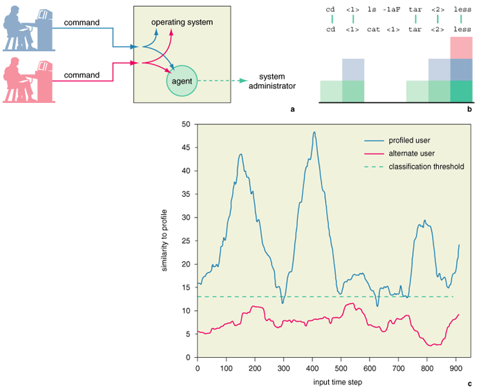
By detecting anomalous patterns in logs of computer usage, a data-mining system can flag suspicious events for system administrators, thus greatly reducing the burden on them. Such a system monitors a single user's computer or account and develops a profile of that user's typical behavior. It can detect anomalies (potentially harmful or abusive actions) as deviations from the known and expected patterns. At the same time, it must be flexible enough to accept differences resulting from "normal" changes—for example, alterations in behavior as a user learns to use a new program or undertakes new tasks.
In an anomaly-detection system that we have developed at Purdue, we represent user behaviors as sequences of commands and their arguments. The sequences are of fixed length (typically 10 elements or "words") and are intended to represent short groups of actions that the user performs frequently. For example, the system may notice that, when writing an article, a user often executes the following sequence of UNIX commands:
cd work/
ls -laF
cd article/
vi myfile.tex
latex myfile.tex
(meaning: move to the work directory; list all files with their sizes, owners, file permissions and last modifications; move to the article directory; edit "myfile.tex" with the editor vi; process "myfile.tex" as a LaTeX file). This sequence would then be recorded and stored in the user's profile. Once the profile is created, the anomaly detector continuously compares the current input command sequences to the known profile to obtain a "similarity" score. If the similarity falls below a certain threshold, the behavior is flagged as anomalous.
Aaron Cox
Just as the heart of a decision-tree algorithm is the evaluation of splitting rules, the heart of this anomaly-detection algorithm is the function used to compare current inputs to the profile. Our approach scores the similarity of two sequences both by the number of identical "words" and by the proximity of those matches. Intuitively, people tend to work at a task contiguously, rather than in fragments. Therefore, we expect that matches occurring in unbroken runs are more likely to represent similar behaviors, whereas matches separated by mismatches are more likely to have happened by chance. As shown in Figure 5b, the first element in an unbroken run of matches adds one point to the similarity score; the next adds two points, and so on. This biases the score toward adjacent matches, because it attributes more importance to each match in a run as the run grows longer. When a run is interrupted, the weight of an individual match is reset to one.
As rudimentary as this method is, it can differentiate users with surprising accuracy. In Figure 5c, the upper curve represents normal computer usage by the profiled user, whereas the lower curve is generated by a different user. Both users were graduate students in Purdue's Machine Learning research laboratory, and their behavioral data were collected as they performed their normal classwork and research tasks. The profile was generated from approximately a month and a half's data, whereas the tested data (displayed in the plot) was drawn from a later period of approximately three months. We have found that the methods discussed here can identify the profiled user with as high as 99 percent accuracy and differentiate the profiled user from an another user almost 94 percent of the time.
Because usage patterns change over time, we included one more stage in our anomaly-detection system. After the system identifies a user as valid, that user's activity is fed back into his or her profile, thereby enabling the system to learn new behavior. Although this improves the system's ability to adapt over time, it does leave the system open to a particularly insidious form of attack known as hostile training. In this attack, an intruder masquerades as a valid user, performing innocuous actions for a time, but gradually engaging in more dangerous activities in an effort to train the defense system to believe the hostile actions are normal. To date, this attack appears to be purely hypothetical, because real adaptive security systems are still rare. But hostile training is a clear danger to such systems, and it is better to design defenses now than wait for the problem to surface when it really matters.
By the way, we were not able to find out exactly how CitiBank caught Levin; they are understandably wary of publishing all the details. A little more is known about another data-mining system, IBM's Fraud and Abuse Management System (FAMS), which has been used to detect millions of dollars of health-care fraud. This system separates routine billing patterns from unusual ones by profiling providers against one another and checking for unusual patterns that have pointed to fraud in the past. For example, Empire Blue Cross and Blue Shield, a health-insurance company in New York, caught a doctor who billed them more than $1.4 million for bronchoscopies that were never performed. The program noticed that the doctor claimed to perform one operation per patient per week, and flagged it as unusual because bronchoscopy is a procedure that is ordinarily done no more than once or twice in a patient's lifetime.
As tectonic plates are to earth and craters are to the moon, so volcanoes are to Venus—the geological feature that, more than any other, influences the planet's history. On earth, tectonic-plate movement provides a fairly smooth way for heat to escape from within the planet, and huge amounts of energy are released into the sea at the plate boundaries. On Venus, there is no plate structure and no ocean to act as a heat sink. Thus the surface is peppered with volcanoes. By studying them, planetary scientists hope to answer such questions as how old the surface is (relatively new, judging from the paucity of craters) and how much heat is escaping from the planet's center.
NASA
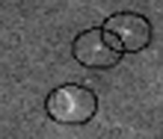
Between 1990 and 1994, NASA's Magellan probe mapped 98 percent of Venus's surface, returning 30,000 synthetic-aperture-radar images. Each of these is a black-and-white, 1024 x 1024 grid of pixels. Volcanoes take on many different appearances: Some are obviously conical (like Mount Rainier), whereas others look more like arcs of white cutting through a cone (like Mount St. Helens after the eruption blew out its side).
Spotting large volcanoes is easy. But cataloguing the small ones, which may be less than a mile—or about 20 pixels—in diameter, is a little bit like counting pieces of hay in a haystack. To automate the process, scientists at NASA's Jet Propulsion Laboratory (JPL) in Pasadena, California, turned to a multi-tiered data-mining algorithm. Each tier processes the volcano candidates from the previous tier with increasing computational power. In this way, the algorithm does not waste time processing regions with no volcanoes, and spends more time on the regions that are more likely to contain a volcano.
Although this method proved very successful at finding volcanoes, JPL's baseline system had one drawback: It used a single volcano template, constructed by averaging the training data. In effect, it assumed that all volcanoes look roughly the same. We were able to improve the true detection rate in the first tier of JPL's algorithm by applying two techniques known as spoiling and clustering.
NASA
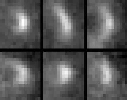
In JPL's training data, the Magellan images are cut into image patches 15 pixels wide by 15 pixels high. Planetary scientists have examined each of these patches to produce a consensus on which features represent volcanoes. The original JPL algorithm produced a composite image by averaging the brightness of each pixel in all the volcanoes (after centering each volcano in its frame, and adjusting for the brightness of the background). Our clustering algorithm separated the volcanoes into six groups—a number determined by the automated procedure—and then traded volcanoes among groups in such a way as to maximize the similarity among members of a given group and minimize the similarity among different groups.
The clustering algorithm would have been computationally infeasible, however, if we had treated every pixel in the 15 x 15 image patch as a significant feature. In the most extreme case, none of the volcanoes in our training set would have been similar enough to cluster together. This problem could have been solved by making the training set sufficiently large to allow meaningful groups to form. But training data are a limited resource, requiring a great deal of human time and expertise to produce. Therefore it made more sense to apply a data-reduction method that recognizes that not every pixel, even in a 15 x 15 picture, is meaningful.
Our approach radically scaled down or "spoiled" the image before clustering. Specifically, we averaged groups of pixels together into a 2 x 3-pixel image, and then used those pixel values as the features for clustering. We chose to reduce the image more in the vertical direction than the horizontal because the volcanos were illuminated from the horizontal direction, so that direction contained more intensity information.
This procedure is called spoiling because it is irreversible—a 15 x 15 image cannot be reconstructed from a 2 x 3 one. But after we grouped the 2 x 3 images into clusters, it was easy enough to retrieve all the original 15 x 15 image patches for each cluster. We averaged the images in each cluster together to form prototype volcanoes (called "matched filters"). These prototypes, not the reduced 2 x 3 versions, were then used to detect volcanoes in the tens of thousands of Magellan images. During the detection phase, each matched filter was compared to each 15 x 15 patch in the image being searched. When the correlation between an image patch and a matched filter exceeded a certain threshold (determined empirically from the training images), the patch was identified as a candidate volcano and passed along to the second tier of the JPL algorithm.
The goal of JPL's first tier was to detect every volcano that is actually present on the planet, but with as few bogus detections as possible. To evaluate our approach, we applied a testing method called cross-validation, which is often used when the amount of ground truth available for testing is small. With 36 images labeled by experts (each containing approximately 16 volcanoes), we trained each algorithm on 30 of the images and then tested it on the other six; we repeated the procedure six times, dividing up the same 36 images into a different set of 30 training and 6 test images. In the cross-validation tests, the multiple matched filters achieved a 100 percent volcano detection rate with fewer false positives than a single filter, and in some cases achieved a 100 percent detection rate when the single filter did not.
This application of KDD to scientific image analysis illustrates two of the key challenges in applying data-mining techniques. The first is to ensure that a method is computationally feasible. The second is to define the relevant features that the data-mining algorithm will consider.
The field of knowledge discovery in databases has emerged in the past five years, bringing together investigators from artificial intelligence, neural networks, statistics, databases and scientific visualization. In industry, the number of commercial tools and consultants has been growing, and they are certain to find a place in science and medicine as well.
We wish to end with a word of caution to any readers who want to apply KDD techniques to their own data sets. KDD can only find patterns in data if the patterns actually exist. Moreover, a successful application of KDD is often an iterative process, in which the KDD expert and the domain expert work together to define the problem and analyze the results.
This research has been carried out with the support of the Jet Propulsion Laboratory under Grant #960628, of IBM under Grant #6712757 and of NASA under Grant #NAG5-6971. Terran Lane's research was supported by the U.S. Department of Defense. The research on land-cover classification was carried out jointly with Mark Friedl from the Center for Remote Sensing at Boston University.
Click "American Scientist" to access home page

American Scientist Comments and Discussion
To discuss our articles or comment on them, please share them and tag American Scientist on social media platforms. Here are links to our profiles on Twitter, Facebook, and LinkedIn.
If we re-share your post, we will moderate comments/discussion following our comments policy.