Getting Your Quarks in a Row
By Brian Hayes
A tidy lattice is the key to computing with quantum fields
A tidy lattice is the key to computing with quantum fields

DOI: 10.1511/2008.75.450
The theories known as QED and QCD are the mismatched siblings of particle physics. QED, or quantum electrodynamics, is the hard-working, conscientious older brother who put himself through night school and earned a degree in accounting. QED describes all the electromagnetic phenomena of nature, and it does so with meticulous accuracy. Calculations carried out within the framework of QED predict properties of the electron to within a few parts per trillion, and those predictions agree with experimental measurements.
QCD, or quantum chromodynamics, is the brilliant but erratic young rebel of the family, who ran off to a commune and came back with tattoos. The theory has the same basic structure as QED, but instead of electrons it applies to quarks; it describes the forces that bind those exotic entities together inside protons, neutrons and other subatomic particles. By all accounts QCD is a correct theory of quark interactions, but it has been a stubbornly unproductive one. If you tried using it to make quantitative predictions, you were lucky to get any answers at all, and accuracy was just too much to ask for.
Now the prodigal theory is finally developing some better work habits. QCD still can't approach the remarkable precision of QED, but some QCD calculations now yield answers accurate to within a few percent. Among the new results are some thought-provoking surprises. For example, QCD computations have shown that the three quarks inside a proton account for only about 1 percent of the proton's measured mass; all the rest of the mass comes from the energy that binds the quarks together. We already knew that atoms are mostly empty space; now we learn that the nuclei inside atoms are mere puffballs, with almost no solid substance.
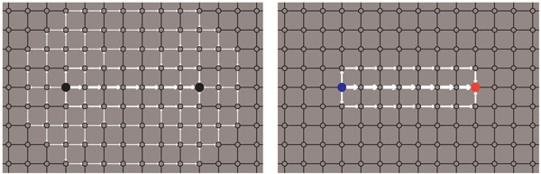
These and other recent findings have come from a computation-intensive approach called lattice QCD, which imposes a gridlike structure on the space and time inhabited by quarks. In this artificial rectilinear microcosm, quarks exist only at the nodes, or crosspoints, of the lattice, and forces act only along the links between the nodes. That's not the way real spacetime is constructed, but the fiction turns out to be helpful in getting answers from QCD. It's also helpful in understanding what QCD is all about.
Bring two electrons close together, and they repel each other. Nineteenth-century theories explained such effects in terms of fields, which are often represented as lines of force that emanate from an electron and extend throughout space. The field produced by each particle repels other particles that have the same electric charge and attracts those with the opposite charge.
QED is a quantum field theory, and it takes a different view of the forces between charged particles. In QED electrons interact by emitting and absorbing photons, which are the quanta, or carriers, of the electromagnetic field. It is the exchange of photons that accounts for attractive and repulsive forces. Thus all those ethereal fields permeating the universe are replaced by localized events—namely the emission or absorption of a photon at a specific place and time. The theory allows for some wilder events as well. A photon—a packet of energy—can materialize to create an electron and its antimatter partner, a positron (e–e+). In the converse event an e–e+ pair annihilates to form a photon.
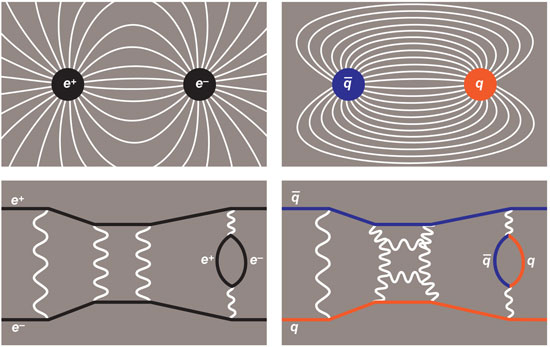
QCD is also a quantum field theory; it describes the same kinds of events, but with a different cast of characters. Where QED is a theory of electrically charge particles, QCD applies to particles that have a property called color charge (hence the name chromodynamics). And forces in QCD are transmitted not by photons but by particles known as gluons, the quanta of the color field.
Yet QCD is not just a version of QED with funny names for the particles. There are at least three major differences between the theories. First, the electric charges of QED come in just two polarities (positive and negative), but there are three varieties of color charge (usually labeled red, green and blue). Second, the photons that carry the electromagnetic force are themselves electrically neutral; gluons not only carry the color force but also have color of their own. As a result, gluons respond to the very force they carry. Finally, the color force is intrinsically stronger than electromagnetism. The strength is measured by a numerical coupling constant, α, which is less than 0.01 for electromagnetism. The corresponding constant for color interactions, αc, is roughly 1.
These differences between QED and QCD have dramatic consequences. Electromagnetism follows an inverse-square law: The force between electrically charged particles falls off rapidly with increasing distance. In contrast, the force between color-charged quarks and gluons remains constant at long distances. Furthermore, it's quite a strong force, equal to about 14 tons. A constant force means the energy needed to separate two quarks grows without limit as you pull them apart. For this reason we never see a quark in isolation; quarks are confined to the interior of protons and neutrons and the other composite particles known as hadrons.
A theory in physics is supposed to be more than just a qualitative description; you ought to be able to use it to make predictive calculations. For example, Newton's theory of gravitation predicts the positions of planets in the sky. Likewise QED allows for predictive calculations in its realm of electrons and photons.
Suppose you want to know the probability that a photon will travel from one point to another. For calculations of this kind Richard Feynman introduced a scheme known as the sum-over-paths method. The idea is to consider every possible path the photon might take and then add up contributions from each of the alternatives. This is rather like booking an airplane trip from Boston to Seattle. You could take a direct flight, or you might stop over in Chicago or Minneapolis—or maybe even Buenos Aires. In QED, each such path is associated with a number called an amplitude; the overall probability of getting from Boston to Seattle is found by summing all the amplitudes, then squaring the result and taking the absolute value. The trick here is that the amplitudes are complex numbers—with real and imaginary parts—which means that in the summing process some amplitudes cancel others. (Another complication is that a photon has infinitely many paths to choose from, but there are mathematical tools for handling those infinities.)
A more elaborate application of QED is calculating the interaction between two electrons: You need to sum up all the ways that the electrons could emit and absorb photons. The simplest possibility is the exchange of a single photon, but events involving two or more photons can't be ruled out. And a photon might spontaneously produce an e–e+ pair, which could then recombine to form another photon. Indeed, the variety of interaction mechanisms is limitless. Nevertheless, QED can calculate the interaction probability to very high accuracy. The key reason for this success is the small value of the electromagnetic coupling constant α. For events with two photons, the amplitude is reduced by a factor of α2, which is less than 0.0001. For three photons the coefficient is α4, and so on. Because these terms are very small, the one-photon exchange dominates the interaction. This style of calculation—summing a series of progressively smaller terms—is known as a perturbative method.
In principle, the same scheme can be applied in QCD to predict the behavior of quarks and gluons; in practice, it doesn't work out quite so smoothly. One problem comes from the color charge of the gluons. Whereas a photon cannot emit or absorb another photon, a gluon, being charged, can emit and absorb gluons. This self-interaction multiplies the number of possible pathways. An even bigger problem is the size of the color-force coupling constant αc. Because this number is close to 1, all possible gluon exchanges make roughly the same contribution to the overall interaction. The single-gluon event can still be taken as the starting point for a calculation, but the subsequent terms are not small corrections; they are just as large as the first term. The series doesn't converge; if you were to try summing the whole thing, the answer would be infinite.
In one respect the situation is not quite as bleak as this analysis suggests. It turns out that the color coupling constant αcisn't really a constant after all. The strength of the coupling varies as a function of distance. The customary unit of distance in this realm is the fermi, equal to 1 femtometer, or 10–15 meter; a fermi is roughly the diameter of a proton or a neutron. If you measure the color force at distances of less than 0.001 fermi, αc dwindles away to only about 0.1. The "constant" grows rapidly, however, as the distance increases. As a result of this variation in the coupling constant, quarks move around freely when they are close together but begin to exert powerful restraining forces as their separation grows. This is the underlying mechanism of quark confinement.
Because the color coupling gets weaker at short distances, perturbative methods can be made to work at close range. In an experimental setting, probing a particle at close range requires high energy. Thus perturbative QCD can tell us about the behavior of quarks in the most violent environments in the universe—such as the collision zones at the Large Hadron Collider now revving near Geneva. But the perturbative theory fails if we want to know about the quarks in ordinary matter at lower energy.
Understanding the low-energy or long-range properties of quark matter is the problem that lattice QCD was invented to address, starting in the mid-1970s. A number of physicists had a hand in developing the technique, but the key figure was Kenneth G. Wilson, now of Ohio State University. It's not an accident that Wilson had been working on problems in solid-state physics and statistical mechanics, where many systems come equipped with a natural lattice, namely that of a crystal.
Introducing an artificial lattice of discrete points is a common strategy for simplifying physical problems. For example, models for weather forecasting establish a grid of points in latitude, longitude and altitude where variables such as temperature and wind direction are evaluated. In QCD the lattice is four-dimensional: Each node represents both a point in space and an instant in time. Thus a particle standing still in space hops along the lattice parallel to the time axis.
It needs to be emphasized that the lattice in QCD is an artificial construct, just as it is in a weather model. No one is suggesting that spacetime really has such a rectilinear gridlike structure. To get rigorous results from lattice studies, you have to consider the limiting behavior as the lattice spacing a goes to zero. (But there are many interesting approximate results that do not require taking the limit.)
One obvious advantage of a lattice is that it helps to tame infinities. In continuous spacetime, quarks and gluons can roam anywhere; even with a finite number of particles, the system has infinitely many possible states. If a lattice has a finite number of nodes and links, the number of quark-and-gluon configurations has a definite bound. In principle, you can enumerate all states.
As it turns out, however, the finite number of configurations is not the biggest benefit of introducing a lattice. More important is enforcing a minimum dimension—namely the lattice spacing a. By eliminating all interactions at distances less than a, the lattice tames a different and more pernicious type of infinity, one where the energy of individual interactions grows without bound.
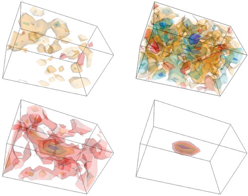
The most celebrated result of lattice QCD came at the very beginning. The mathematical framework of QCD itself (without the lattice) was formulated in about 1973; this work included the idea that quarks become "asymptotically free" at close range and suggested the hypothesis of confinement at longer range. Just a year later Wilson published evidence of confinement based on a lattice model. What he showed was that color fields on the lattice do not spread out in the way that electromagnetic fields do. As quarks are pulled apart, the color field between them is concentrated in a narrow "flux tube" that maintains a constant cross section. The energy of the flux tube is proportional to its length. Long before the tube reaches macroscopic length, there is enough energy to create a new quark-antiquark pair. The result is that isolated quarks are never seen in the wild; only collections of quarks that are color-neutral can be detected.
When I first heard about lattice QCD, I found the idea instantly appealing. Other approaches to particle physics require mastery of some very challenging mathematics, but the lattice methods looked like something I could get a grip on—something discrete and finite, where computing the state of a quantum system would be a matter of filling in columns and rows of numbers.
Those early hopes ended in disappointment. I soon learned that lattice QCD does not bring all of quantum field theory down to the level of spreadsheet arithmetic. There is still heavy-duty mathematics to be done, along with a great deal of heavy-duty computing. Nevertheless, I continue to believe that the lattice version of the weird quantum world is easier to grasp than any other. My conviction has been reinforced by the discovery of an article, "Lattice QCD for Novices," published 10 years ago by G. Peter Lepage of Cornell University. Lepage doesn't offer lattice QCD in an Excel spreadsheet, but he does present an implementation written in the Python programming language. The entire program fits in a page or two.
Lepage's lattice model for novices has just one space dimension as well as a time dimension; in other words, it describes particles moving back and forth along a line segment. And what the program simulates isn't really a quantum field theory; there are no operators for the creation and annihilation of particles. All the same, reading the source code for the program gives an inside view of how a lattice model works, even if the model is only a toy.
At the lowest level is a routine to generate thousands of random paths, or configurations, in the lattice, weighted according to their likelihood under the particular rule that governs the physical evolution of the system. Then the program computes averages for a subset of the configurations, as well as quantities that correspond to experimentally observable properties, such as energy levels. Finally, more than half the program is given over to evaluating the statistical reliability of the results.
Going beyond toy programs to research models is clearly a big step. Lepage writes of the lattice method:
Early enthusiasm for such an approach to QCD, back when QCD was first invented, quickly gave way to the grim realization that very large computers would be needed....
It's not hard to see where the computational demand comes from. A lattice for a typical experiment might have 32 nodes along each of the three spatial dimensions and 128 nodes along the time dimension. That's roughly 4 million nodes altogether, and 16 million links between nodes. Gathering a statistically valid sample of random configurations from such a lattice is an arduous process.
Some lattice QCD simulations are run on "commodity clusters"—machines assembled out of hundreds or thousands of off-the-shelf computers. But there is also a long tradition of building computers designed explicitly for lattice computations. The task is one that lends itself to highly parallel architectures; indeed, one obvious approach is to build a network of processors that mirrors the structure of the lattice itself.
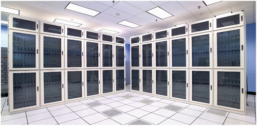
Photograph courtesy of Brookhaven National Laboratory.
One series of dedicated machines is known as QCDOC, for QCD on a chip. The chip in question is a customized version of the IBM PowerPC microprocessor, with specialized hardware for interprocessor communication. Some 12,288 processors are organized in a six-dimensional mesh, so that each processor communicates directly with 12 nearest neighbors. Three such machines have been built, two at Brookhaven National Laboratory and the third at the University of Edinburgh.
The QCDOC machines were completed in 2005, and attention is now turning to a new generation of special-purpose processors. Ideas under study include chips with multiple "cores," or subprocessors, and harnessing graphics chips for lattice calculations.
Meanwhile, algorithmic improvements may be just as important as faster hardware. The computational cost of a lattice QCD simulation depends critically on the lattice spacing a; specifically, the cost scales as 1/a6. For a long time the conventional wisdom held that a must be less than about 0.1 fermi for accurate results. Algorithmic refinements that allow a to be increased to just 0.3 or 0.4 fermi have a tremendous payoff in efficiency. If a simulation at a=0.1 fermi has a cost of 1,000,000 (in some arbitrary units), the same simulation at a=0.4 costs less than 250.
With growing computational resources and algorithmic innovations, QCD finally has the power to make sharp, quantitative predictions. An exemplary case is a recent careful calculation of quark masses.
The importance of these masses is noted in a review article by Andreas S. Kronfeld of the Fermi National Accelerator Laboratory. The two lightest quarks, designated u and d, are the constituents of protons and neutrons. (The proton is uud and the neutron udd.) Patterns among the masses of other quarks suggest that u should weigh more than d. If that were the case, a u could decay into a d. "But then protons would decay into neutrons, positrons and neutrinos.... This universe would consist of neutron stars surrounded by a swarm of photons and neutrinos, and nothing else," Kronfeld says. Since the actual universe exhibits a good deal more variety, we can infer that the d must be heavier than the u. Until recently, however, QCD simulations could not produce reliable or accurate estimates of the u and d masses.
Earlier lattice computations had to ignore a crucial aspect of QCD. Events or pathways in which quark-antiquark pairs are created or annihilated were simply too costly to compute, and so they were suppressed in the simulations. This practice yields acceptable results for some QCD phenomena, but pair-creation events have a major influence on other properties, including estimates of the quark masses.
Algorithmic refinements developed in the past decade have finally allowed quark-antiquark contributions to be included in lattice computations. The new quark-mass estimates based on these methods were made by Quentin Mason, Howard D. Trottier, Ron Horgan, Christine T. H. Davies and Lepage. They derive a u mass of 1.9 MeV (million electron-volts) and a d mass of 4.4 MeV (with estimated systematic and statistical errors of about 8 percent). Thus the uud quarks in a proton weigh about 8 MeV; the mass of the proton itself is 938 MeV.
I am intrigued by this result, and I admire the heroic effort that produced it. On the other hand, I confess to a certain puzzlement that it takes so much effort to pin down a few of the simple numbers that define the universe we live in. Nature, after all, seems to compute these values effortlessly. Why is it such hard work for us?
©Brian Hayes
Click "American Scientist" to access home page
American Scientist Comments and Discussion
To discuss our articles or comment on them, please share them and tag American Scientist on social media platforms. Here are links to our profiles on Twitter, Facebook, and LinkedIn.
If we re-share your post, we will moderate comments/discussion following our comments policy.